Accuracy Modelling
One broad numeracy score with probe effects is supported over separate sub-skill scores
1 Why this matters
↑ IRT State of Play · Response Process · Speed & Profiles
Before scoring students on this screener, we need to answer a foundational question: does the accuracy evidence support one broad numeracy score, or separate sub-skill scores?
If performance on number-line, magnitude comparison, and other tasks is driven by a single underlying numeracy ability, one overall score is appropriate. If there are genuinely distinct sub-skills — spatial number sense vs. symbolic comparison, say — then separate profile scores could give teachers more actionable information.
This page tests the structure of the accuracy-based numeracy score by comparing three structural IRT models. All models are fitted by marginal maximum likelihood (MML): the EM algorithm for the simpler structures, and the MHRM stochastic approximation for the multidimensional model.
Note
Relationship to A2. The structure-comparison evidence supports the same design choice used in A2: report one broad numeracy achievement score with probe/testlet effects absorbed as nuisance structure. The structure-comparison codes M0-struct, M1-struct, M3-struct (always shown in fixed-width to avoid collision) are not the M0/A1/A2/A3 codes used in the IRT State of Play. A2 is the Stan implementation of the winning structure found here.
2 Three candidate models
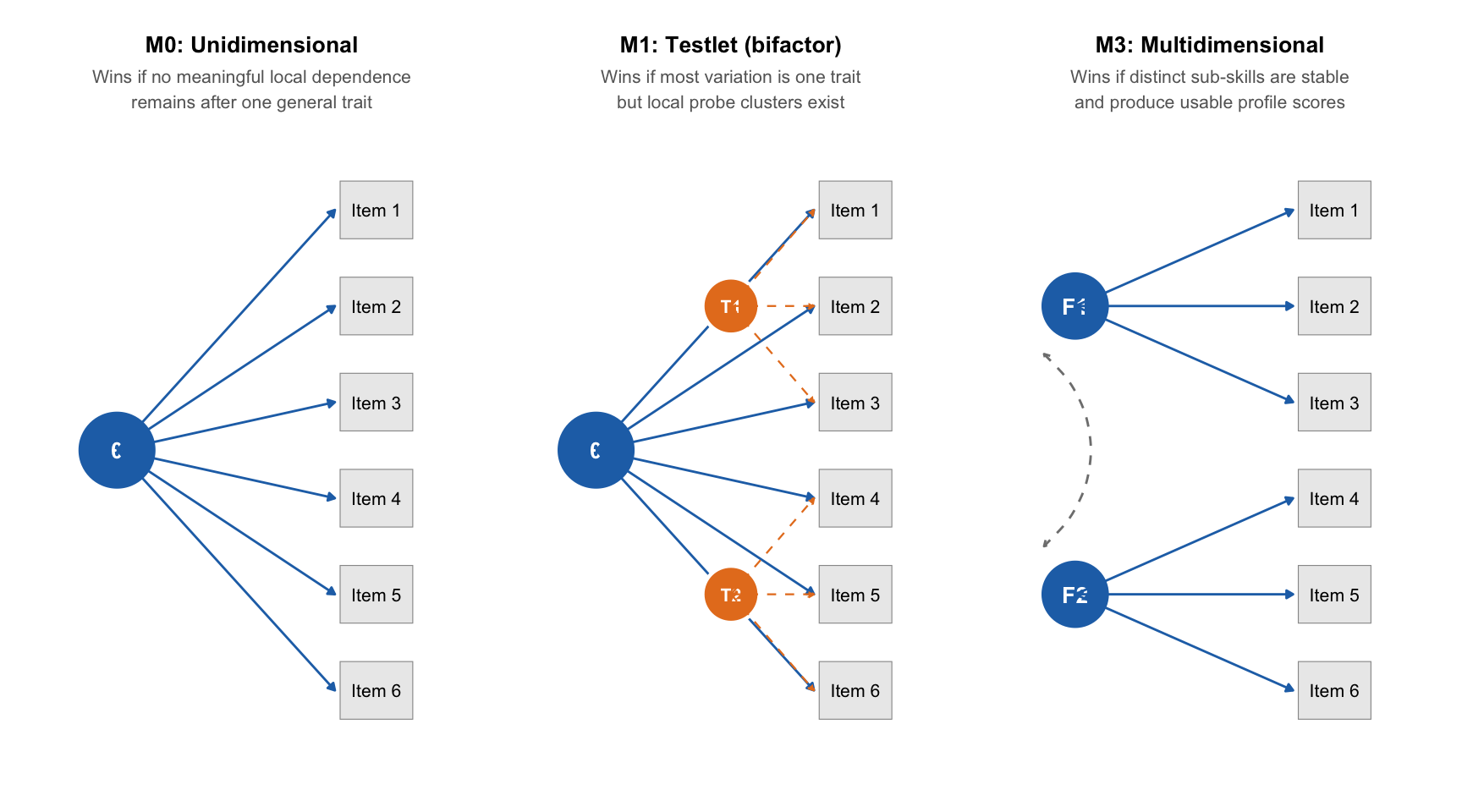
The three models represent increasingly complex accounts of what drives student responses. The internal IDs M0-struct, M1-struct, M3-struct are used only within this analysis and are not the M0/A1/A2/A3 codes in the IRT State of Play.
| Plain label | Internal ID | Structure | Preferred if... |
|---|---|---|---|
| Single achievement trait | M0-struct | One latent numeracy trait drives all items | No meaningful local dependence or sub-skill structure exists |
| Single trait + probe effects | M1-struct | One general trait plus a testlet residual for each probe cluster | Most variation is one trait, but items within a probe are more similar than expected |
| Separate sub-skill traits | M3-struct | Separate correlated factors, one per task domain | Distinct sub-skills are stable enough to produce usable profile scores |
2.1 Model equations
All three models share the same item response functions and differ only in how they parameterise the latent trait(s). Binary items use a Rasch model (slope constrained to 1). Number-line items use the generalised partial credit model (GPCM) with an estimated discrimination parameter. The number-line categorisation policy is documented separately in Number-Line PCM Policy.
Binary items (Rasch):
\[P(Y_{ij} = 1 \mid \theta_i, b_j) = \text{logit}^{-1}(\theta_i - b_j)\]
Number-line items (GPCM, \(k \in \{0,1,2\}\)): continuous number-line scores are categorised as <0.85, 0.85–<0.95, and >=0.95 in the current structure-comparison run.
\[P(Y_{ij} = k \mid \theta_i, b_j, a_j, d_{j,\cdot}) \propto \exp\!\left(\sum_{c=1}^{k} a_j(\theta_i - b_j - d_{j,c})\right)\]
where \(b_j\) is item location, \(a_j\) is the estimated discrimination (GPCM items only), and \(d_{j,c}\) are ordered step thresholds.
All three structures are fitted by marginal maximum likelihood (MML): the EM algorithm for M0-struct and M1-struct; the MHRM stochastic approximation for M3-struct. The IRT development models on the State of Play page (A2, A3, joint models) are fitted by HMC in Stan. Estimation differences do not threaten the structure-comparison conclusion: BIC margins here are large (thousands of points) and replicate across terms and sample definitions, so the winning structure is not an artefact of the MML/HMC choice.
M0-struct — Single achievement trait. A single latent trait \(\theta_i\) enters all item response functions directly.
M1-struct — Single trait + probe effects. A general trait \(\theta_i\) loads on every item. Each probe cluster \(t\) contributes an additional testlet residual \(s_{t,i}\), orthogonal to \(\theta_i\):
\[\text{logit}\,P(Y_{ij} = 1) = \theta_i + s_{t(j),i} - b_j\]
Both \(\theta_i\) and \(s_{t,i}\) have slope = 1 (Rasch constraint). The testlet residual absorbs local dependence within a probe without splitting the reported achievement score.
M3-struct — Separate sub-skill traits. Each item loads on a single domain factor \(\theta_{f,i}\):
\[\text{logit}\,P(Y_{ij} = 1) = \theta_{f(j),i} - b_j\]
Factors are allowed to correlate, but only where student overlap between domains is sufficient (minimum 80 students with responses to both factor groups, and at least 10% of the possible overlap). There is no general factor; all cross-domain covariation is captured through the pairwise correlations that pass the overlap gate.
3 How subtests map to dimensions
M3-struct with a separate factor for every task was not computationally feasible on the main pooled units. We therefore collapsed number-line tasks (BNL, UNLC, UNLNC) into a single NL factor and magnitude comparison & missing number tasks (MC, MNA, MNC) into a single SYM_MAG factor. Match quantity and decomposition variants each keep their own factor. A cohort-level unit has 4 factors (NL, SYM_MAG, one MQ variant, one DMT variant); pooled units combining both exam groups have 6. The diagram below shows all tasks grouped by test family.
Warning: The `label.size` argument of `geom_label()` is deprecated as of ggplot2 3.5.0.
ℹ Please use the `linewidth` argument instead.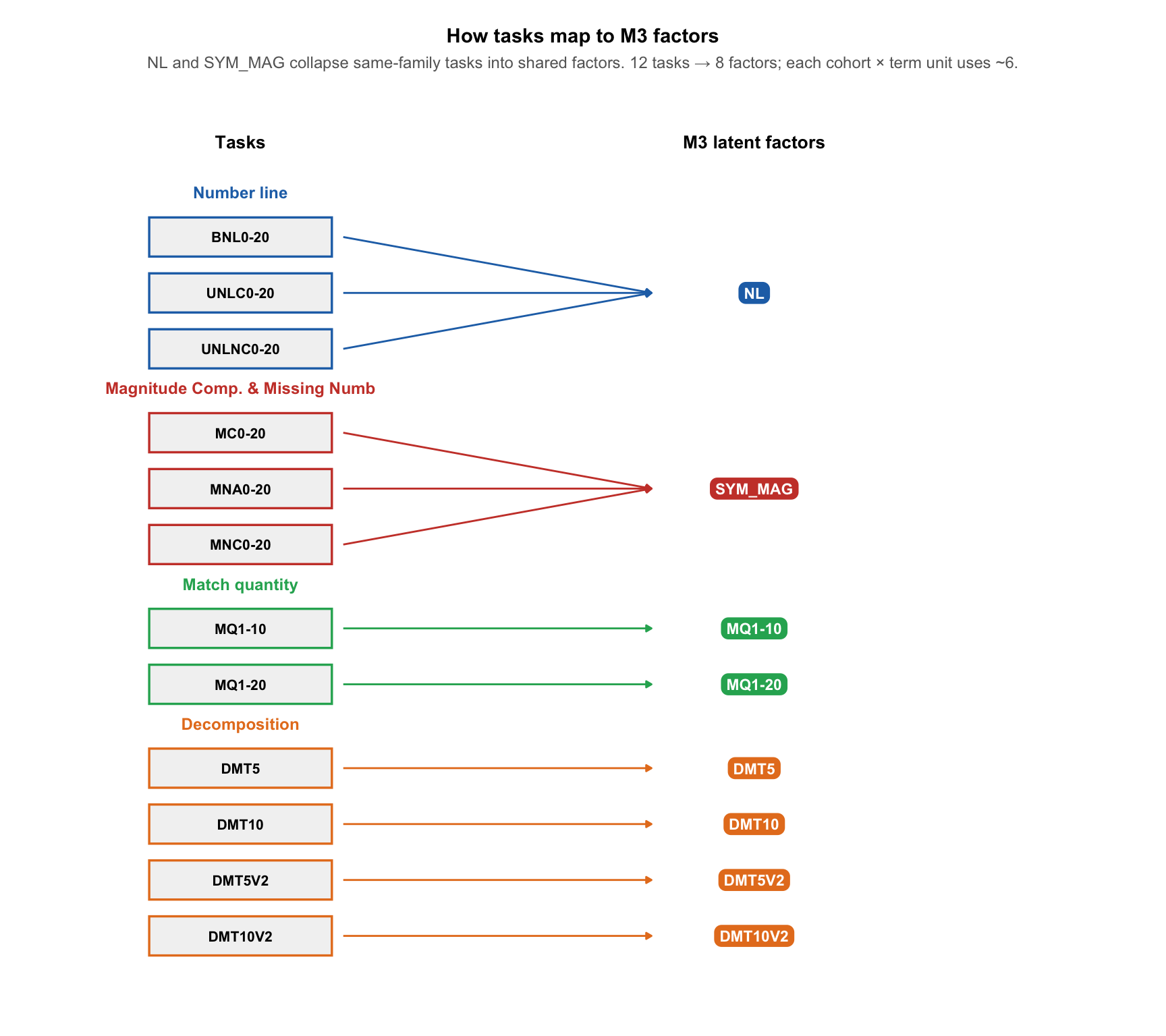
4 What the evidence shows
The comparison ran in two stages. The initial run (foundation_parallel_20260206) fitted all three structures across 12 units (2 terms × 2 sample definitions × 3 cohort scopes) — but M3-struct was not computationally feasible on the four main pooled units and timed out there. A full-N robustness run (foundation_fulln_boot4_prod_20260209) then completed the M1-struct vs M3-struct comparison on the four main pooled units and added bootstrap stability checks. Both runs agree: the single-trait-plus-probe-effects structure is preferred.
The primary criterion is BIC (fit versus complexity) computed from the model log-likelihood and number of non-missing item responses. Secondary checks are residual local dependence (Q3) and school-level bootstrap resampling.
4.1 BIC comparison
The analysis was run across units representing every combination of term (Term 1 and Term 4), sample definition (“All students” = every student with at least 5 attempted items in that term; “Stable schools” = only students from the 39 schools present in both terms), and cohort scope (Foundation A, Foundation B, or all foundation students pooled).
BIC penalises model complexity: a lower BIC means the model explains the data better relative to its number of free parameters.
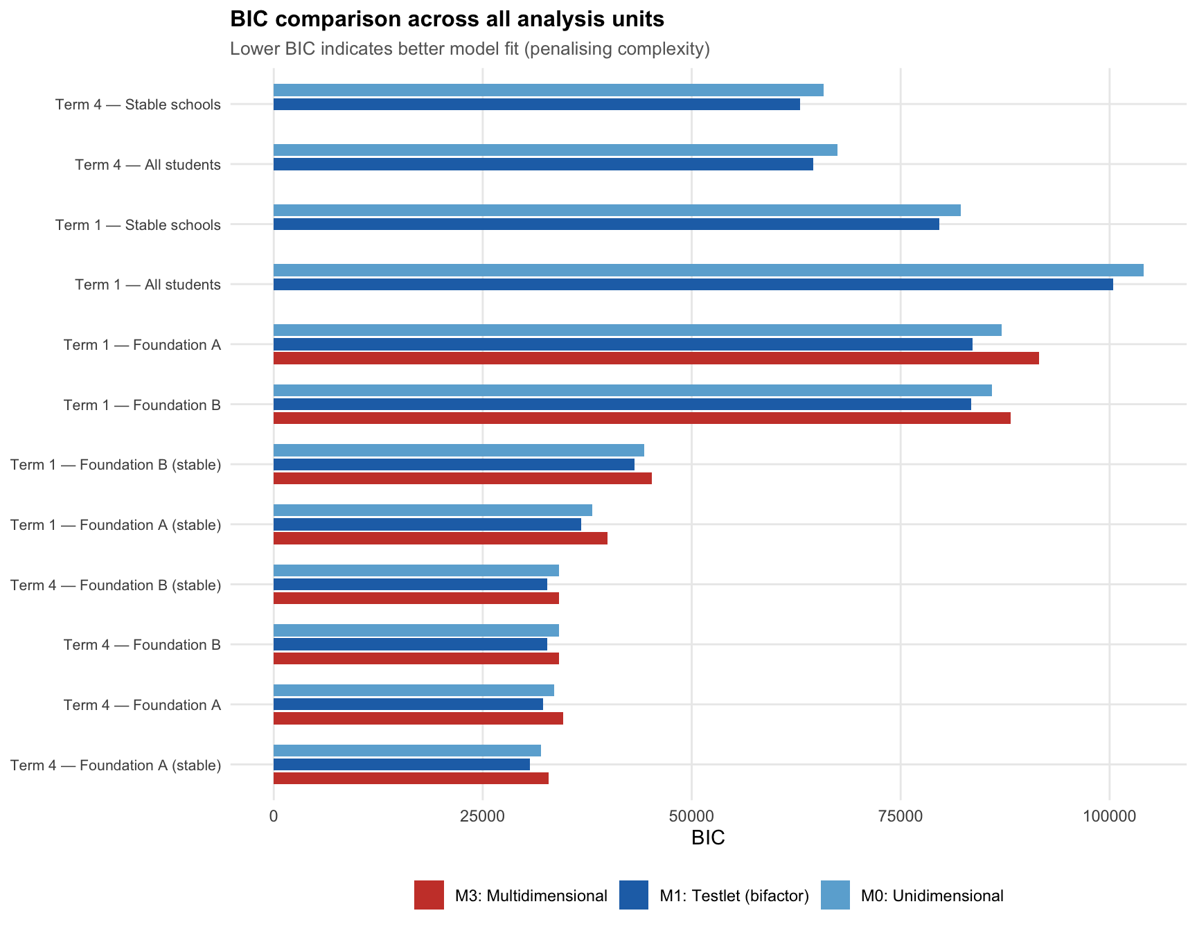
Single trait + probe effects wins in every unit. Across all 12 analysis units — both terms, both sample definitions, all cohorts — the probe-effects structure achieves the lowest BIC. The single-trait-no-effects structure consistently ranks second, and the separate-sub-skills structure ranks last.
4.2 Head-to-head BIC differences
To quantify the margin of victory, we examine pairwise BIC differences between models. A negative value in “M1 vs M0” means M1 fits better; a positive value in “M3 vs M1” means M1 fits better than M3.
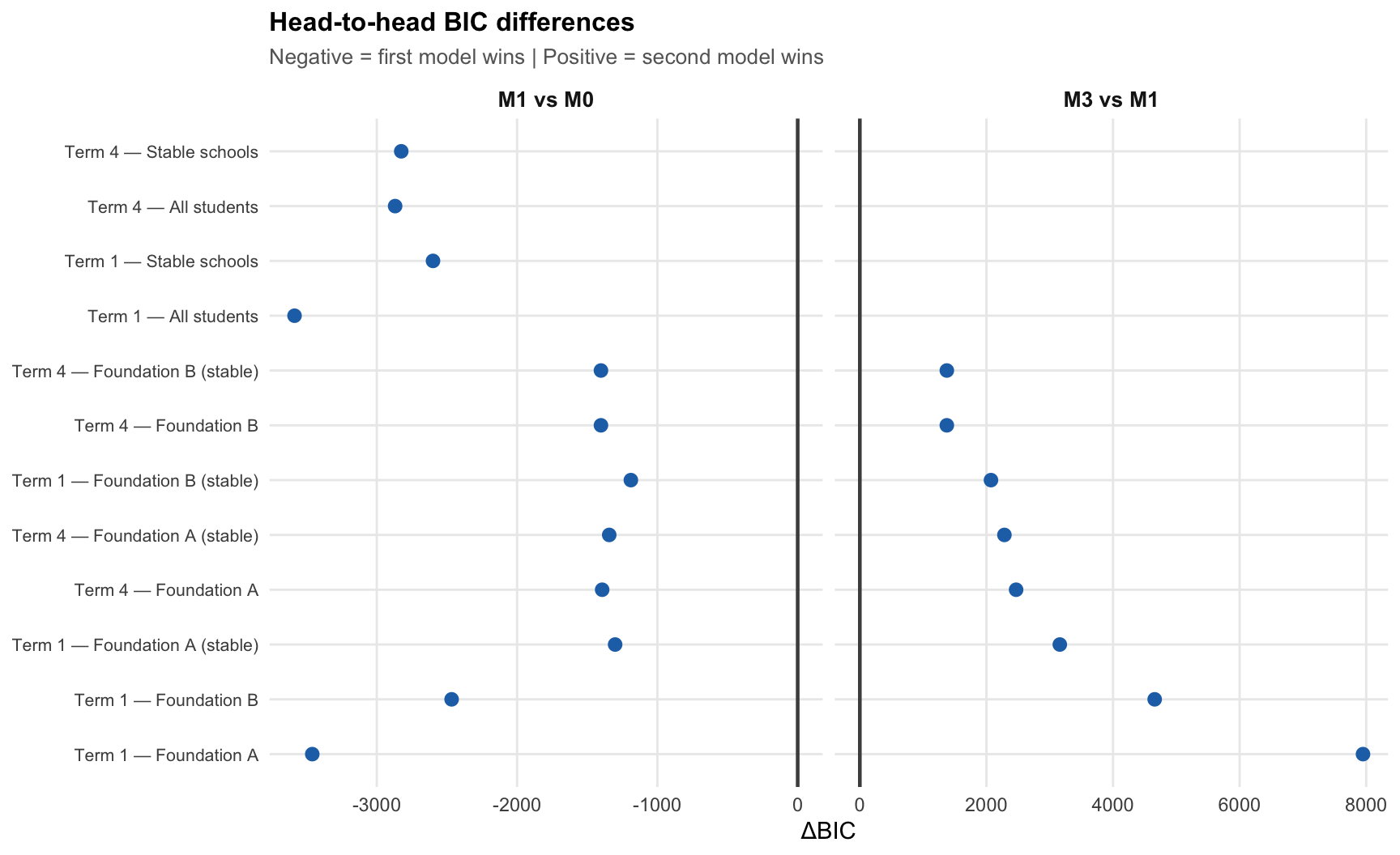
Adding probe effects to a single trait consistently improves fit over the single-trait-alone model, while the separate-sub-skills model is consistently worse than the probe-effects model — often by thousands of BIC points.
4.3 Bootstrap stability
Could these results be an artefact of the particular school sample? To check, we resampled schools 30 times per slice (with replacement) and refit both M1 and M3 on each bootstrap sample. The slices range from approximately 1,100 to 2,500 students; stable-school slices draw from the 39 schools present in both terms.
| Slice | N students | N observations | N schools |
|---|---|---|---|
| Term 1 — All students | 2,514 | 152,068 | — |
| Term 1 — Stable schools | 1,186 | 71,289 | 39 |
| Term 4 — All students | 1,098 | 68,371 | — |
| Term 4 — Stable schools | 1,076 | 67,039 | 39 |
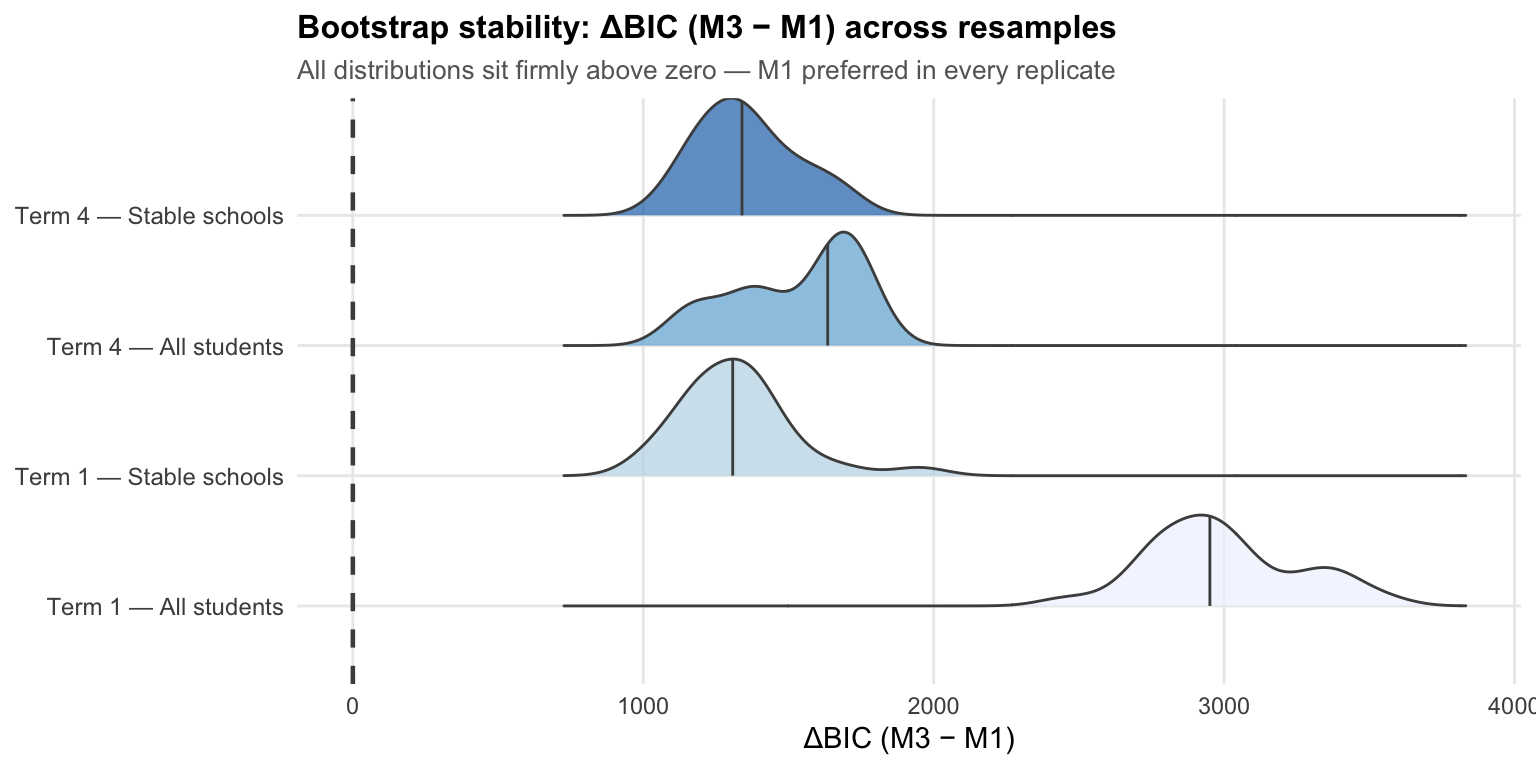
Each ridge shows the distribution of ΔBIC across 30 bootstrap replicates. All four distributions sit entirely above zero — even the most conservative replicate favours the single-trait-plus-probe-effects structure by over 1,000 BIC points. The wider spread for Term 4 — All students reflects the smaller sample (1,098 students vs 2,514 in Term 1).
4.4 Residual dependence (Q3)
The Q3 statistic measures unexplained local dependence between item pairs after accounting for the latent structure. Lower values indicate the model has adequately captured the correlation structure.
| Scope | Model | Units | Median mean abs(Q3) | Median prop abs(Q3) > threshold |
|---|---|---|---|---|
| By cohort | Single achievement trait | 8 | 0.1051 | 0.1424 |
| By cohort | Single trait + probe effects | 8 | 0.0940 | 0.1146 |
| By cohort | Separate sub-skill traits | 8 | 0.1200 | 0.1804 |
| All students | Single achievement trait | 4 | 0.1130 | 0.1573 |
| All students | Single trait + probe effects | 4 | 0.1028 | 0.1355 |
The probe-effects structure achieves the lowest residual dependence across both scopes: it absorbs local probe-cluster effects that the single-trait-alone structure leaves unexplained, and does so more efficiently than the separate-sub-skills structure.
5 Conclusion
5.1 Single broad score with probe effects is supported
The single-trait-plus-probe-effects structure wins consistently: it achieves the lowest BIC in all 12 analysis units, demonstrates the lowest residual dependence, and its advantage is stable under school-level bootstrap resampling.
What this means for scoring: the accuracy evidence supports reporting one broad numeracy score. Probe/testlet effects should be absorbed as nuisance structure inside the model, not reported as separate sub-skill scores. Separate sub-skill scores — number-line vs. symbolic comparison, for instance — are not ready: the multidimensional structure fits worse and factor-level precision does not meet the minimum thresholds for reporting in any unit tested.
Relationship to A2. This finding supports the A2 model design: one broad numeracy score with probe/testlet random effects. A2 is the Stan implementation of this structure. See the IRT State of Play for A2’s current status.
Looking ahead: as the item pool grows in future assessment cycles, it will be worth revisiting whether distinct sub-skill profiles become feasible. For now, no profile-level scores should be reported to teachers or used operationally.
6 Technical appendix
NoteA1: Full BIC table (all completed units)
| Unit | BIC M0 | BIC M1 | BIC M3 | Δ M0–best | Δ M1–best | Δ M3–best | Winner |
|---|---|---|---|---|---|---|---|
| Term 1 — Foundation A | 87,094.6 | 83,634.9 | 91,584.3 | 3459.7 | 0 | 7949.4 | M1_1d_testlets |
| Term 1 — Foundation B | 85,936.3 | 83,469.7 | 88,127.7 | 2466.6 | 0 | 4658.0 | M1_1d_testlets |
| Term 1 — Foundation A (stable) | 38,089.5 | 36,788.2 | 39,947.5 | 1301.2 | 0 | 3159.2 | M1_1d_testlets |
| Term 1 — Foundation B (stable) | 44,334.2 | 43,145.2 | 45,216.9 | 1189.0 | 0 | 2071.7 | M1_1d_testlets |
| Term 4 — Foundation A | 33,577.8 | 32,184.3 | 34,653.1 | 1393.6 | 0 | 2468.9 | M1_1d_testlets |
| Term 4 — Foundation B | 34,125.4 | 32,723.3 | 34,097.5 | 1402.2 | 0 | 1374.3 | M1_1d_testlets |
| Term 4 — Foundation A (stable) | 31,965.5 | 30,622.2 | 32,906.2 | 1343.3 | 0 | 2284.0 | M1_1d_testlets |
| Term 4 — Foundation B (stable) | 34,125.4 | 32,723.3 | 34,097.5 | 1402.2 | 0 | 1374.3 | M1_1d_testlets |
| Term 1 — All students | 104,043.8 | 100,457.6 | NA | 3586.2 | 0 | NA | M1_1d_testlets |
| Term 1 — Stable schools | 82,192.0 | 79,592.7 | NA | 2599.3 | 0 | NA | M1_1d_testlets |
| Term 4 — All students | 67,401.5 | 64,532.3 | NA | 2869.2 | 0 | NA | M1_1d_testlets |
| Term 4 — Stable schools | 65,799.3 | 62,973.6 | NA | 2825.6 | 0 | NA | M1_1d_testlets |
NoteA2: Residual dependence detail (Q3 by unit and model)
| Unit | Model | Mean abs(Q3) | Max abs(Q3) | Prop abs(Q3) > threshold |
|---|---|---|---|---|
| Term 1 — Foundation A | Single achievement trait | 0.0953 | 0.9828 | 0.1257 |
| Term 1 — Foundation A | Single trait + probe effects | 0.0856 | 0.9977 | 0.1145 |
| Term 1 — Foundation A | Separate sub-skill traits | 0.1220 | 1.0000 | 0.1949 |
| Term 1 — Foundation A (stable) | Single achievement trait | 0.0979 | 1.0000 | 0.1228 |
| Term 1 — Foundation A (stable) | Single trait + probe effects | 0.0890 | 0.7938 | 0.1050 |
| Term 1 — Foundation A (stable) | Separate sub-skill traits | 0.1216 | 0.7943 | 0.1829 |
| Term 4 — Foundation A | Single achievement trait | 0.1047 | 0.9870 | 0.1437 |
| Term 4 — Foundation A | Single trait + probe effects | 0.0931 | 0.9792 | 0.1092 |
| Term 4 — Foundation A | Separate sub-skill traits | 0.1258 | 0.9880 | 0.1841 |
| Term 4 — Foundation A (stable) | Single achievement trait | 0.1074 | 0.9964 | 0.1471 |
| Term 4 — Foundation A (stable) | Single trait + probe effects | 0.0958 | 0.9943 | 0.1146 |
| Term 4 — Foundation A (stable) | Separate sub-skill traits | 0.1265 | 0.9974 | 0.1825 |
| Term 1 — Foundation B | Single achievement trait | 0.1017 | 1.0000 | 0.1335 |
| Term 1 — Foundation B | Single trait + probe effects | 0.0952 | 0.8873 | 0.1274 |
| Term 1 — Foundation B | Separate sub-skill traits | 0.1073 | 0.9454 | 0.1503 |
| Term 1 — Foundation B (stable) | Single achievement trait | 0.1124 | 0.9958 | 0.1645 |
| Term 1 — Foundation B (stable) | Single trait + probe effects | 0.1068 | 0.9619 | 0.1529 |
| Term 1 — Foundation B (stable) | Separate sub-skill traits | 0.1184 | 0.9769 | 0.1784 |
| Term 4 — Foundation B | Single achievement trait | 0.1054 | 1.0000 | 0.1424 |
| Term 4 — Foundation B | Single trait + probe effects | 0.0940 | 0.9554 | 0.1147 |
| Term 4 — Foundation B | Separate sub-skill traits | 0.1030 | 0.9880 | 0.1369 |
| Term 4 — Foundation B (stable) | Single achievement trait | 0.1054 | 1.0000 | 0.1424 |
| Term 4 — Foundation B (stable) | Single trait + probe effects | 0.0940 | 0.9554 | 0.1147 |
| Term 4 — Foundation B (stable) | Separate sub-skill traits | 0.1030 | 0.9880 | 0.1369 |
| Term 1 — All students | Single achievement trait | 0.1268 | 1.0000 | 0.1940 |
| Term 1 — All students | Single trait + probe effects | 0.1180 | 1.0000 | 0.1808 |
| Term 1 — Stable schools | Single achievement trait | 0.1125 | 1.0000 | 0.1542 |
| Term 1 — Stable schools | Single trait + probe effects | 0.1049 | 1.0000 | 0.1445 |
| Term 4 — All students | Single achievement trait | 0.1125 | 1.0000 | 0.1561 |
| Term 4 — All students | Single trait + probe effects | 0.0997 | 0.9941 | 0.1237 |
| Term 4 — Stable schools | Single achievement trait | 0.1136 | 1.0000 | 0.1584 |
| Term 4 — Stable schools | Single trait + probe effects | 0.1007 | 0.9938 | 0.1266 |
NoteA3: Bootstrap quantiles (M3 − M1)
| Slice | Planned reps | Usable reps | Median ΔBIC | P10 ΔBIC | P90 ΔBIC |
|---|---|---|---|---|---|
| Term 1 — All students | 30 | 30 | 2,951.0 | 2,726.8 | 3,379.8 |
| Term 1 — Stable schools | 30 | 28 | 1,308.0 | 1,130.8 | 1,524.9 |
| Term 4 — All students | 30 | 17 | 1,635.0 | 1,194.8 | 1,743.6 |
| Term 4 — Stable schools | 30 | 14 | 1,339.9 | 1,190.2 | 1,585.2 |
| all_slices | 120 | NA | 1,536.3 | 1,183.4 | 3,062.1 |
Positive values throughout confirm M1 is preferred over M3 in every bootstrap replicate. The P10 column shows even the most conservative replicate favours M1 by a large margin.
NoteA4: Run IDs
Three-model comparison run
- Run ID:
foundation_parallel_20260206
Full-N robustness run (bootstrap)
- Run ID:
foundation_fulln_boot4_prod_20260209
| Run | Status | Converged | Count |
|---|---|---|---|
| Full-N robustness | ok | TRUE | 8 |
| Three-model comparison | ok | TRUE | 32 |
| Three-model comparison | timed_out | FALSE | 4 |
NoteA5: Decision criteria
The structural model selection follows a layered decision protocol:
Primary — BIC: the model with the lowest BIC across the majority of analysis units is preferred. BIC is computed from the model log-likelihood and the number of non-missing item responses, and penalises the number of free parameters, guarding against overfitting.
Secondary — Residual dependence (Q3): Yen’s Q3 statistic measures unexplained pairwise item dependence after conditioning on the latent structure. Lower mean |Q3| and a lower proportion of item pairs exceeding the threshold (|Q3| > 0.2) indicate better local-dependence absorption.
Robustness — School-level bootstrap: schools are resampled with replacement (30 replicates per slice) and both M1 and M3 are refit. If the BIC preference reverses in a meaningful proportion of replicates, the result is considered unstable.
Profile gate (secondary): even if a multidimensional model won on fit, profile scores are only reported to teachers if factor-level measurement precision exceeds minimum thresholds (determinacy > 0.80 for teacher-facing scores, > 0.70 for internal use). This gate is currently not met for any M3 factor.
NoteA6: Full decision summary table
“Teacher profile pass” and “Internal profile pass” indicate whether M3’s factor-level precision exceeds minimum thresholds for reporting profile scores (determinacy > 0.80 for teacher-facing, > 0.70 for internal use). All units show FALSE — no M3 factor achieves sufficient precision for profile scores.
| Unit | BIC winner | BIC value | Teacher profile pass | Internal profile pass |
|---|---|---|---|---|
| Term 1 — Foundation A | M1_1d_testlets | 83,634.9 | FALSE | FALSE |
| Term 1 — Foundation A (stable) | M1_1d_testlets | 36,788.2 | FALSE | FALSE |
| Term 4 — Foundation A | M1_1d_testlets | 32,184.3 | FALSE | FALSE |
| Term 4 — Foundation A (stable) | M1_1d_testlets | 30,622.2 | FALSE | FALSE |
| Term 1 — Foundation B | M1_1d_testlets | 83,469.7 | FALSE | FALSE |
| Term 1 — Foundation B (stable) | M1_1d_testlets | 43,145.2 | FALSE | FALSE |
| Term 4 — Foundation B | M1_1d_testlets | 32,723.3 | FALSE | FALSE |
| Term 4 — Foundation B (stable) | M1_1d_testlets | 32,723.3 | FALSE | FALSE |
| Term 1 — All students | M1_1d_testlets | 100,457.6 | FALSE | FALSE |
| Term 1 — Stable schools | M1_1d_testlets | 79,592.7 | FALSE | FALSE |
| Term 4 — All students | M1_1d_testlets | 64,532.3 | FALSE | FALSE |
| Term 4 — Stable schools | M1_1d_testlets | 62,973.6 | FALSE | FALSE |
7 See also
- IRT State of Play — full model-iteration glossary including A2, and the current operational status of all IRT work.
- Number-Line PCM Policy — how continuous number-line scores are converted into ordered GPCM categories.
- Response Process: Completion, Reach, and Response-State Evidence — what response records tell us beyond accuracy.
- Speed Modelling: Accuracy–Speed Profiles — RT modelling and response-process profiles.
- IRT Model - Foundation 2025 Term 1 — original Foundation T1 calibration using the winning structure.