| exam_group_cohort | n_students |
|---|---|
| F-A | 1320 |
| F-B | 1238 |
IRT Model - Foundation 2025 Term 1
Data Quality, Methodology, and Instrument Insights
Executive Summary
This report reviews Foundation Term 1 numeracy screening data, first with model-free exploratory analyses, then with the joint IRT + RT model for accuracy and timed fluency.
Data highlights:
- Students: 2,558 Foundation students in cleaned Term 1 responses after filters (practice/ABR excluded); 2,517 included in the fitted joint model (requires modelled responses/RT).
- Coverage (modelled students): strong per-student coverage (median ~60 accuracy items, ~52 timed RTs).
- Item exposure: moderate inequality (Gini ~0.3–0.4); 36 items with <20 responses flagged for parameter instability.
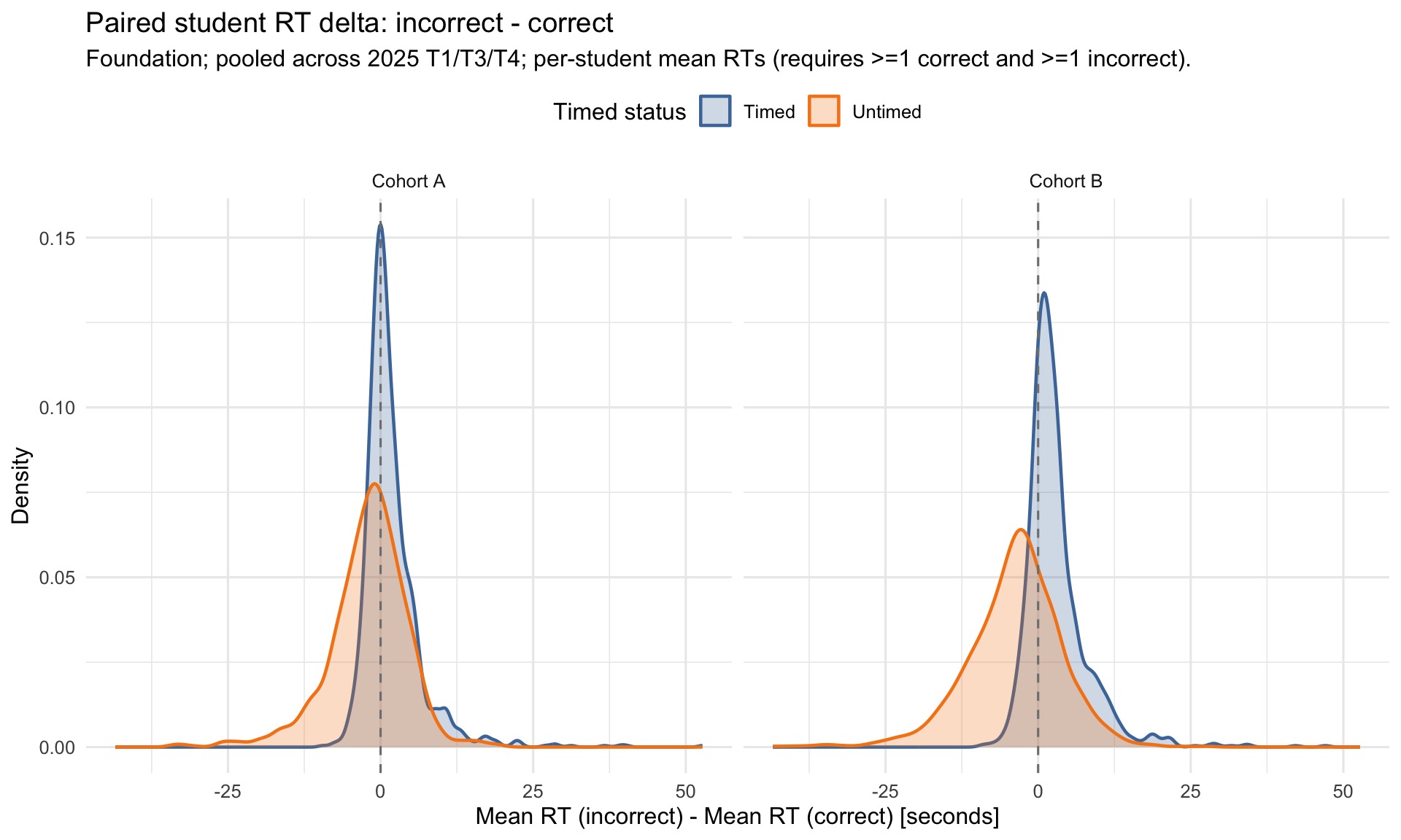
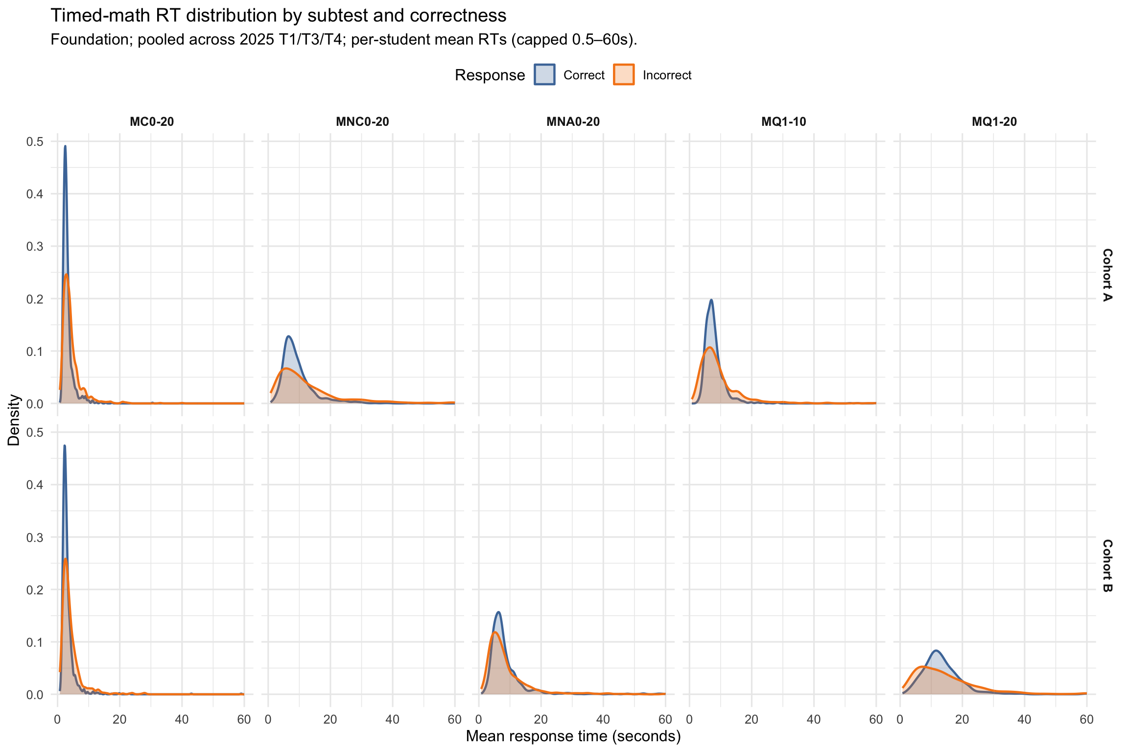
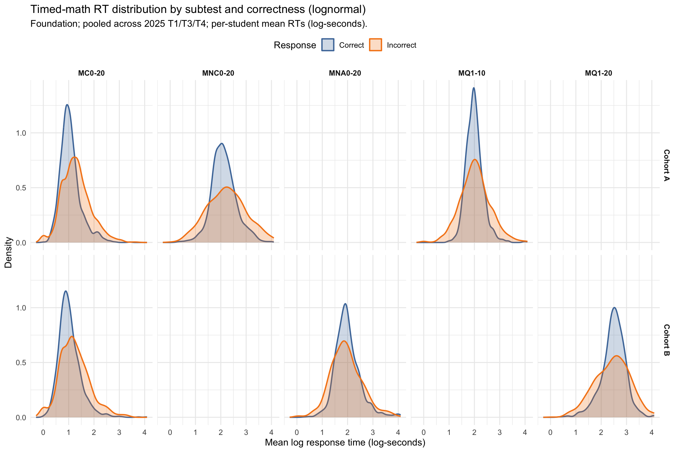
- RT patterns: incorrect responses are faster than correct on timed-math items, consistent with rapid guessing on items beyond ability.
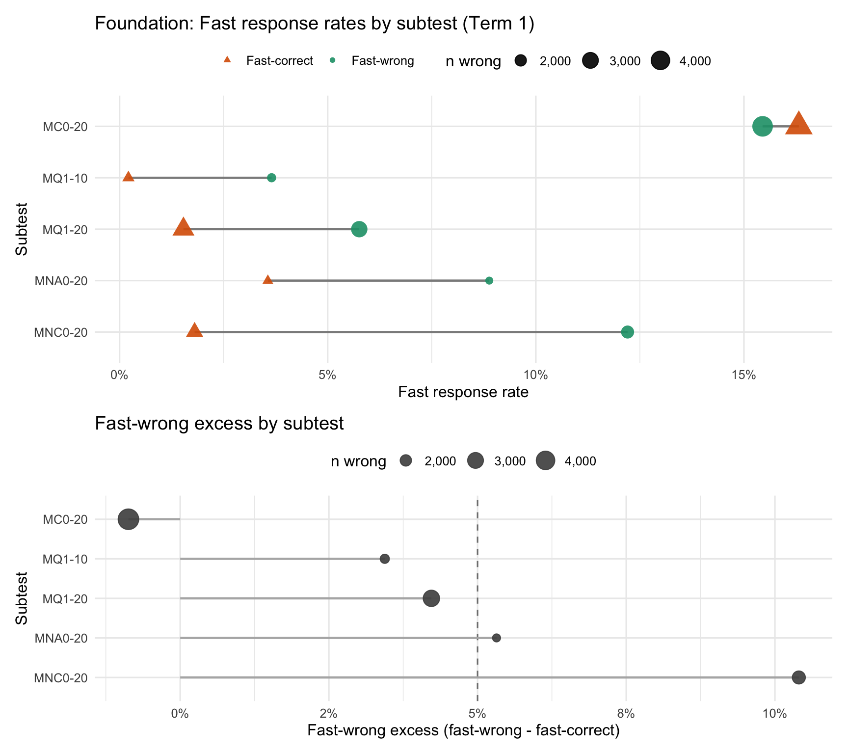
- Fast-wrong signal: substantial fast-wrong excess on MC0-20 and MNC0-20 in particular — exceeds what a lognormal RT model predicts, indicating a rapid-guess subpopulation.
- 60s cap rates: STPM shows the highest rate of hitting the 60-second ceiling, reflecting pause/disengage behaviour.
Model findings:
- Model convergence: clean MCMC (0 divergences; max Rhat ~1.01; E-BFMI min ~0.65).
- Construct validity: θ aligns strongly with observed accuracy; τ_base aligns with STPM RT; τ_math_total aligns with timed-math RT; τ_reg_adj is ~independent of STPM speed.
- Low-information rates: 2.4% of students flagged, driven mainly by low counts rather than unstable posteriors.
- Item QC flags: 36 low-exposure items (<20 responses) and 3/30 NL items with disordered PCM steps (one per NL subgroup).
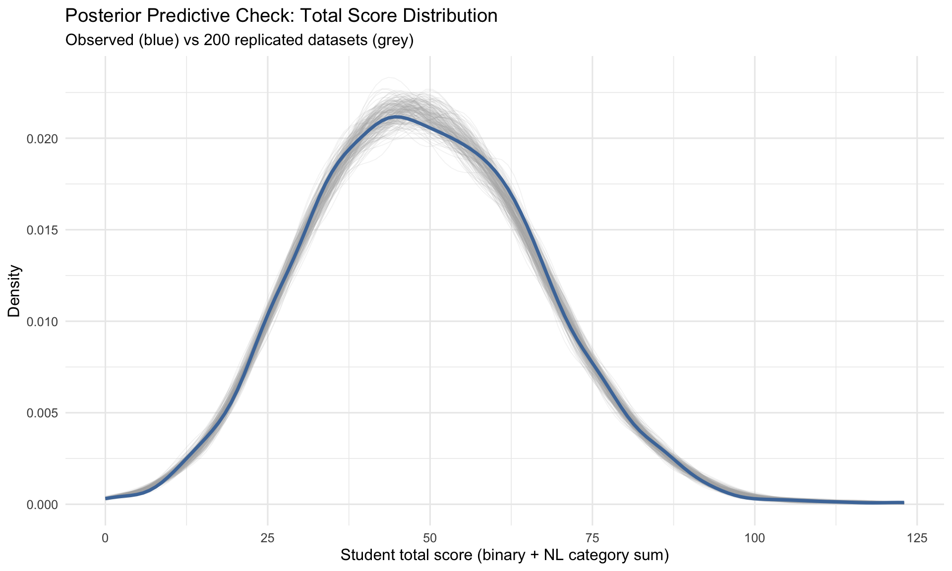
- Accuracy model fit (PPC): strong for binary items (0/184 items outside 90% PI). Total score density matches posterior replications; the mean/SD table shows a small downward shift in observed vs predicted, motivating NL category PPCs and a scoring-parity audit.
- RT model fit (PPC): systematic misfit at the extremes — (a) log-RT p99 tails underpredicted; (b) STPM 60s cap rate exceeds the model’s 90% PI; (c) fast-wrong rates for MC0-20 and MNC0-20 are much higher than predicted. This v3 run uses all timed RTs; next-iteration speed modelling should be probe-aware (e.g., correct-only RT for probes with strong rapid-guess evidence).
1 Data & Cohorts
1.1 Student Counts
Total Foundation students: 2558
Note: the fitted joint model includes a subset of these students (those with modelled accuracy responses and/or timed RT). See Model Diagnostics → Input coverage for the model-included counts.
1.2 Subtest overview
Below are short descriptions of each Foundation subtest (paired A/B forms noted where applicable):
| Subtest | Description |
|---|---|
| BNL0-20 | Bounded number line; place a target number on a 0-20 line with endpoints. |
| UNLC0-20 / UNLNC0-20 | Unbounded number line; place a target using 0 and a unit marker (chairs vs no-chairs variants). |
| MC0-20 | Magnitude comparison; choose the larger of two numbers. |
| MNC0-20 / MNA0-20 | Missing number; MNC = choose the missing number from options, MNA = judge if a sequence is ascending. |
| MQ1-10 / MQ1-20 | Match quantity; match quantity representations to numerals (timed). |
| DMT5 / DMT10 | Decomposition; part-whole hidden quantity, choose how many are hidden (untimed). |
| STPM | Speeded pattern matching; tap the matching picture (baseline speed). |
| Cohort | test_subgroup | subtest_name | n_items | is_timed | typical_distractor_count |
|---|---|---|---|---|---|
| A | BNL0-20 | Bounded Number Line 0-20 | 10 | FALSE | NA |
| A | DMT5 | Decomposition to 5 | 10 | FALSE | 2 |
| A | MC0-20 | Magnitude Comparison 0-20 | 38 | TRUE | 4 |
| A | MNC0-20 | Missing Number Choice 0-20 | 30 | TRUE | 4 |
| A | MQ1-10 | Match Quantity 1-10 | 30 | TRUE | 4 |
| A | STPM | Speeded Pattern Matching | 20 | TRUE | 2 |
| A | UNLNC0-20 | Unbounded Number Line 0-20 (no chairs) | 10 | FALSE | NA |
| B | BNL0-20 | Bounded Number Line 0-20 | 10 | FALSE | NA |
| B | DMT10 | Decomposition to 10 | 10 | FALSE | 2 |
| B | MC0-20 | Magnitude Comparison 0-20 | 44 | TRUE | 4 |
| B | MNA0-20 | Missing Number Ascending 0-20 | 30 | TRUE | 4 |
| B | MQ1-20 | Match Quantity 1-20 | 30 | TRUE | 4 |
| B | STPM | Speeded Pattern Matching | 20 | TRUE | 2 |
| B | UNLC0-20 | Unbounded Number Line 0-20 (chairs) | 10 | FALSE | NA |
1.2.1 Data Filters & Inclusion Criteria
This analysis uses Foundation year level Term 1 data only, excluding practice items (is_practice == TRUE) and abridged version (ABR, is_abr == TRUE).
Important distinction: The dataset contains placeholder rows with is_attempted == FALSE for many items. This does NOT necessarily mean the item was presented to the student. We use gap/tail classification as a proxy for not-reached status:
- Gap missingness:
is_attempted == FALSEwherequestion_no ≤ max(question_no)among attempted items within a subtest - Tail missingness:
is_attempted == FALSEwherequestion_no > max(question_no)among attempted items (likely not reached)
Exploratory data analysis (sections 2–9) uses both attempted and not-attempted rows for missingness analysis. Performance metrics (accuracy, fluency) use attempted rows only.
1.3 Subtest Order
| test_subgroup | F-A | F-B |
|---|---|---|
| BNL0-20 | 1 | 1 |
| STPM | 2 | 2 |
| MQ1-10 | 3 | NA |
| MC0-20 | 4 | 4 |
| DMT5 | 5 | NA |
| MNC0-20 | 6 | NA |
| UNLNC0-20 | 7 | NA |
| MQ1-20 | NA | 3 |
| DMT10 | NA | 5 |
| MNA0-20 | NA | 6 |
| UNLC0-20 | NA | 7 |
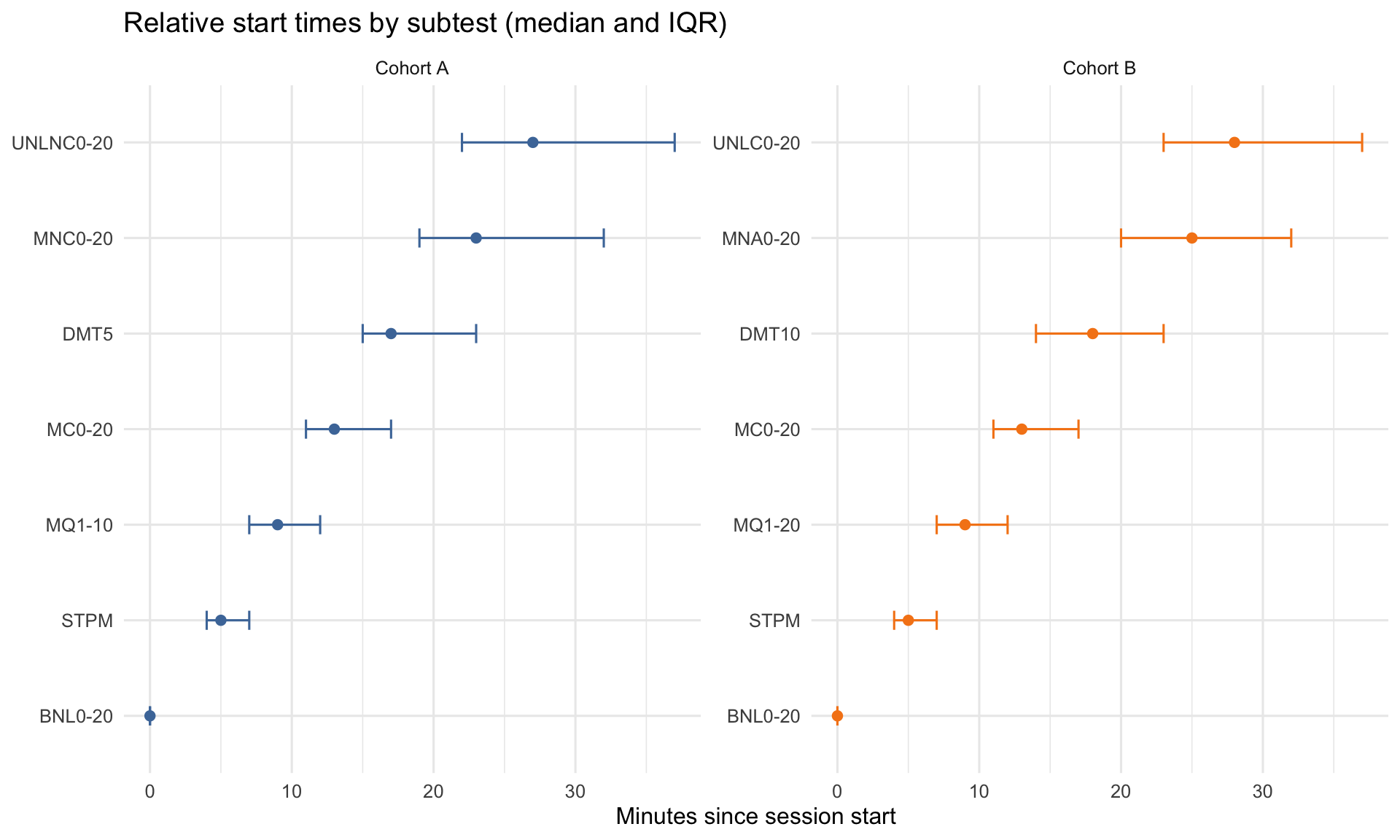
2 Student Coverage and Missingness
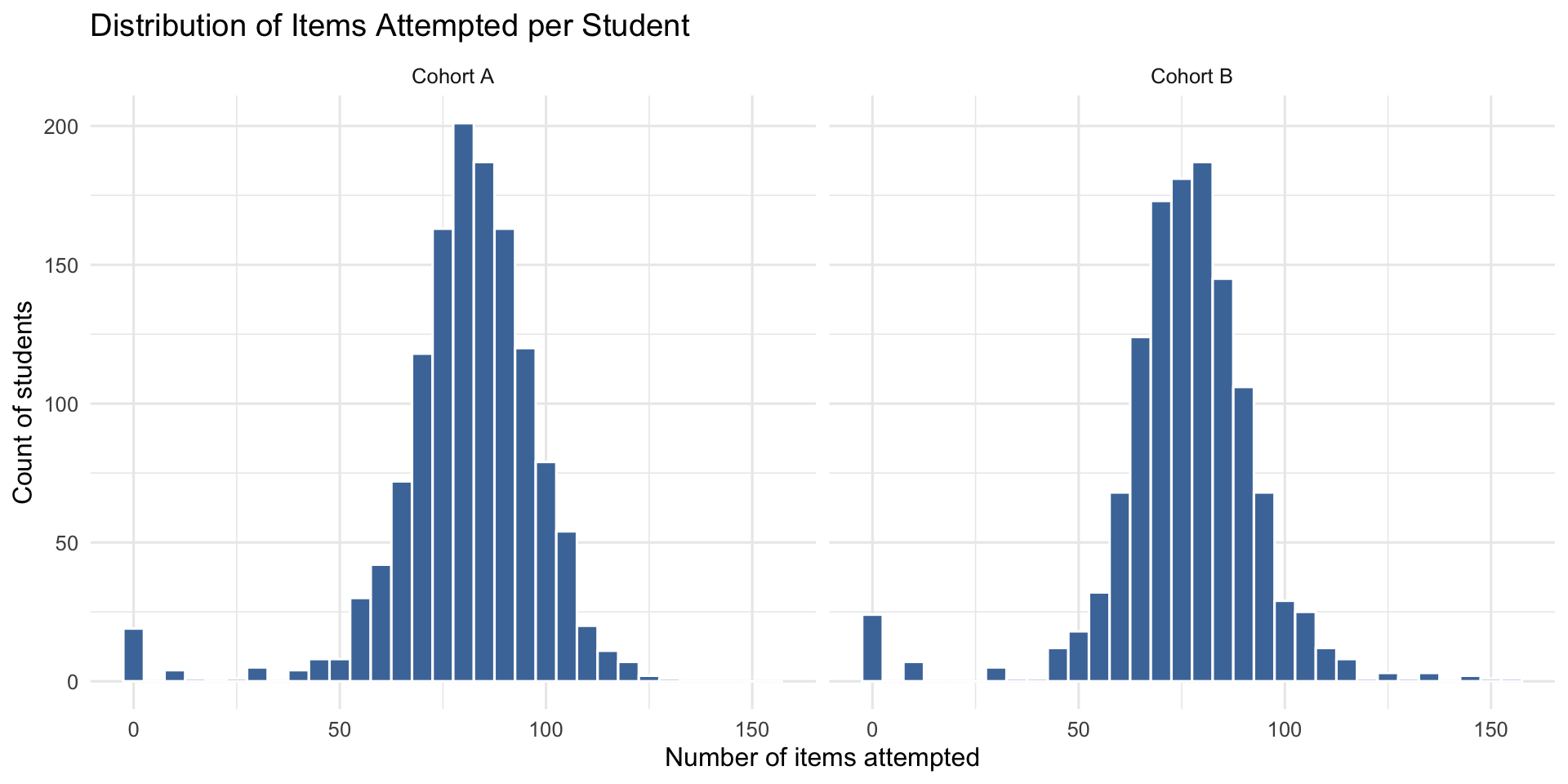
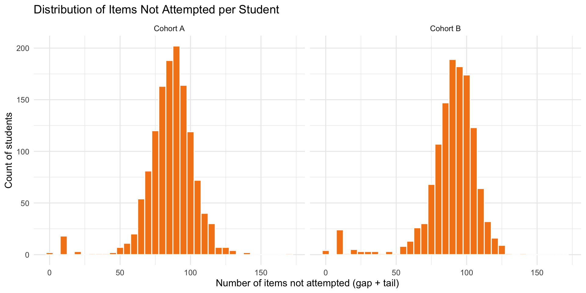
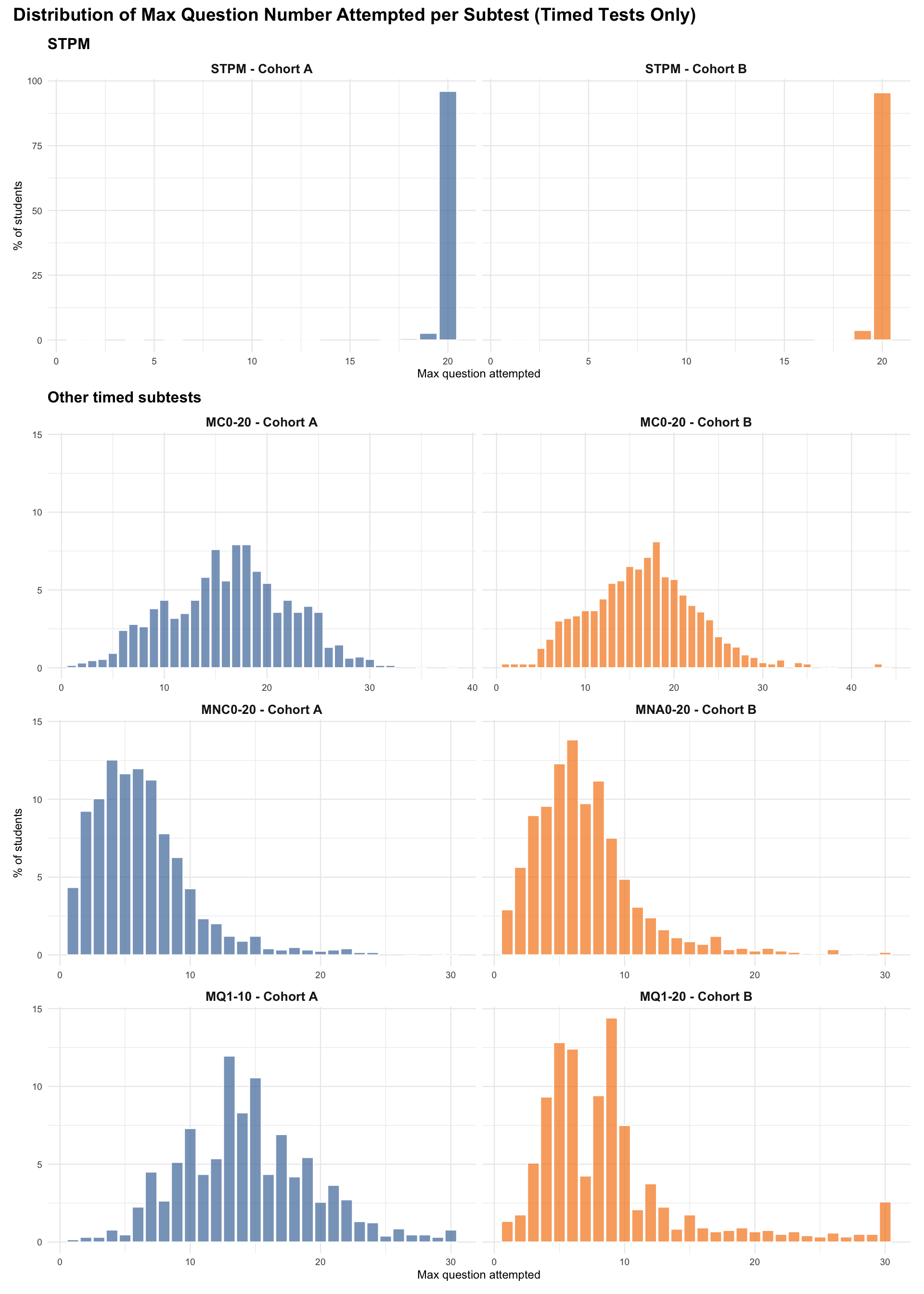
2.1 Item Exposure & Missingness
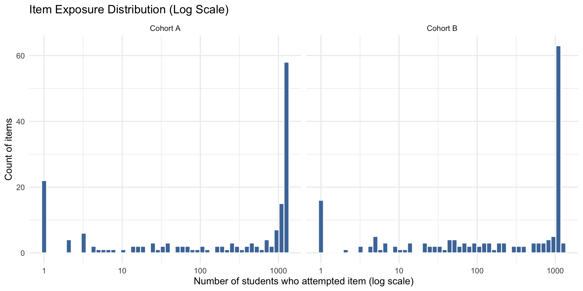
2.1.1 Exposure Inequality (Lorenz Curve & Gini Coefficient)
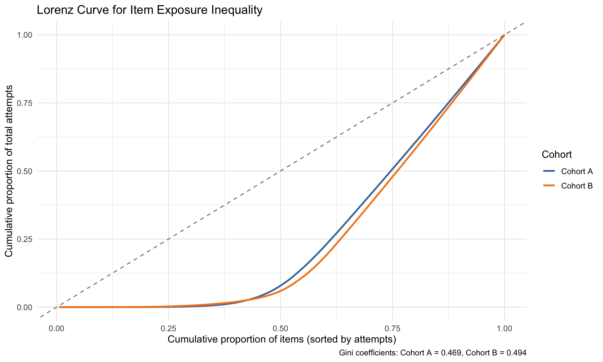
The Lorenz curve shows inequality in item exposure. The dashed diagonal represents perfect equality (all items attempted by the same number of students). The further the curve bows below this line, the greater the inequality. The Gini coefficient quantifies this (0 = perfect equality, 1 = maximum inequality). Higher values indicate some items receive disproportionately more attempts than others.
3 Response Time Analysis
RT Preprocessing for EDA vs Model
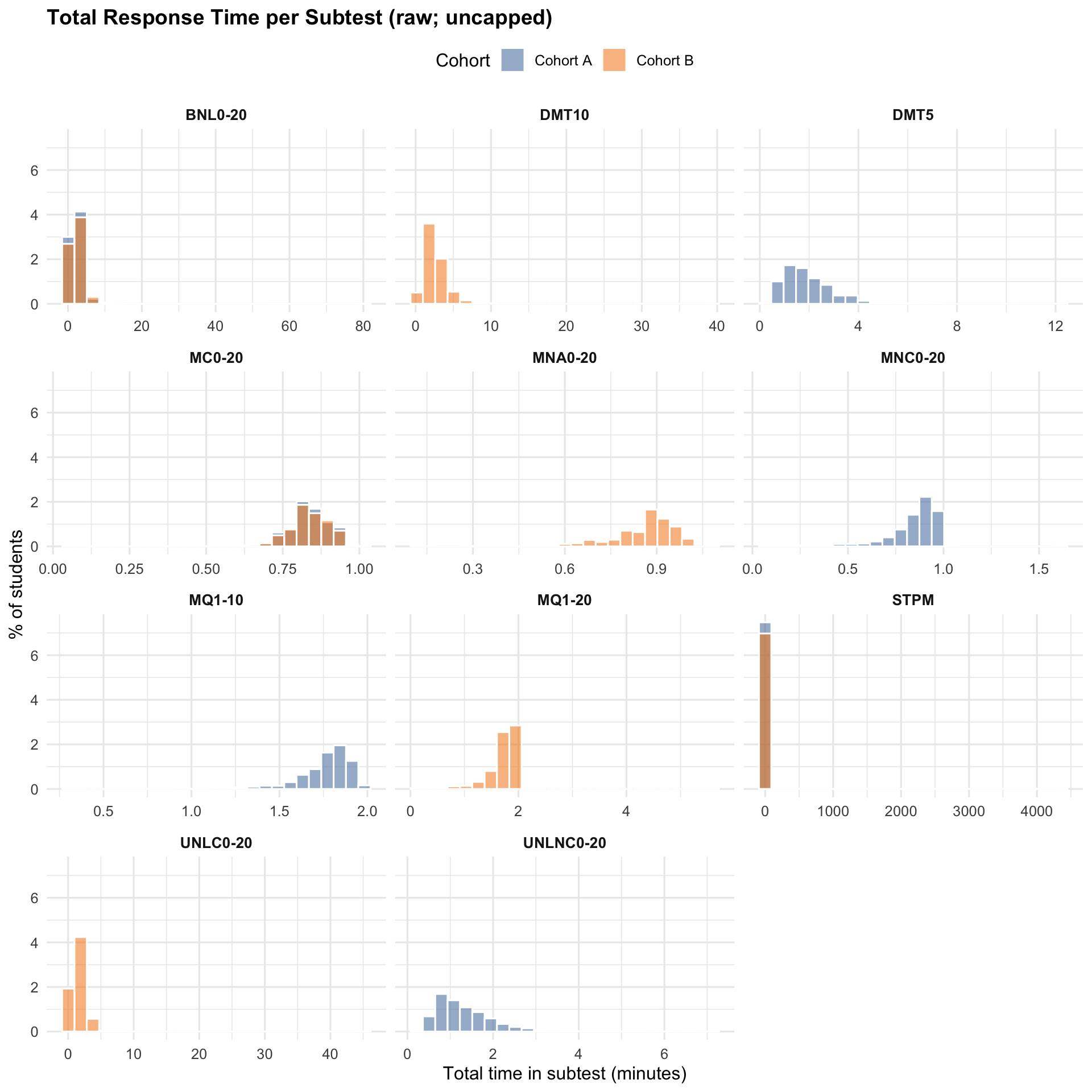
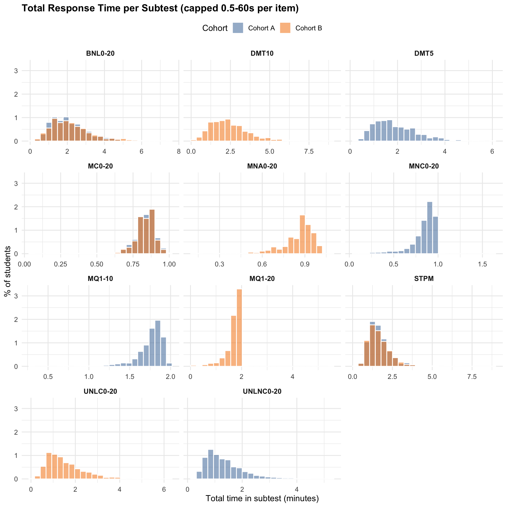
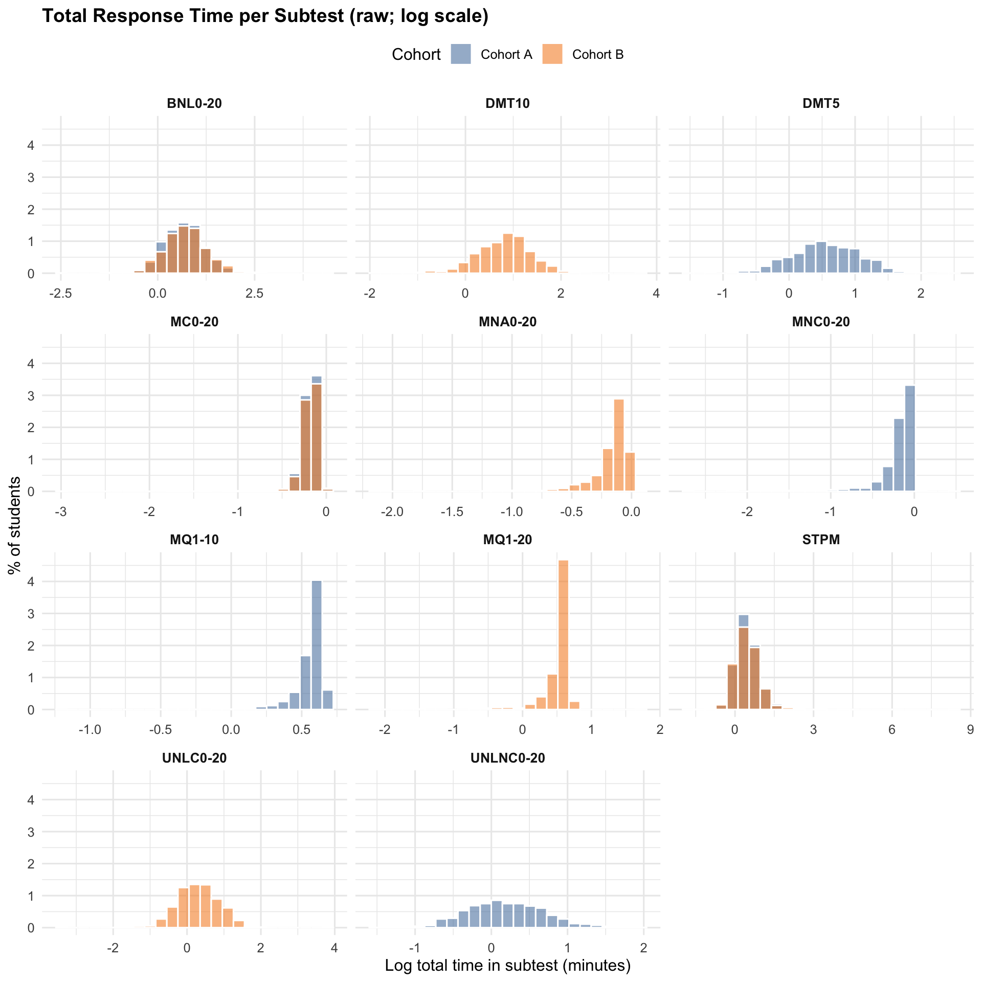
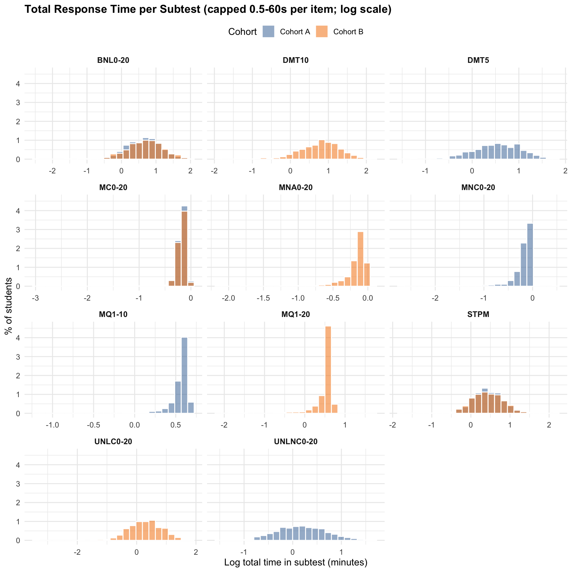
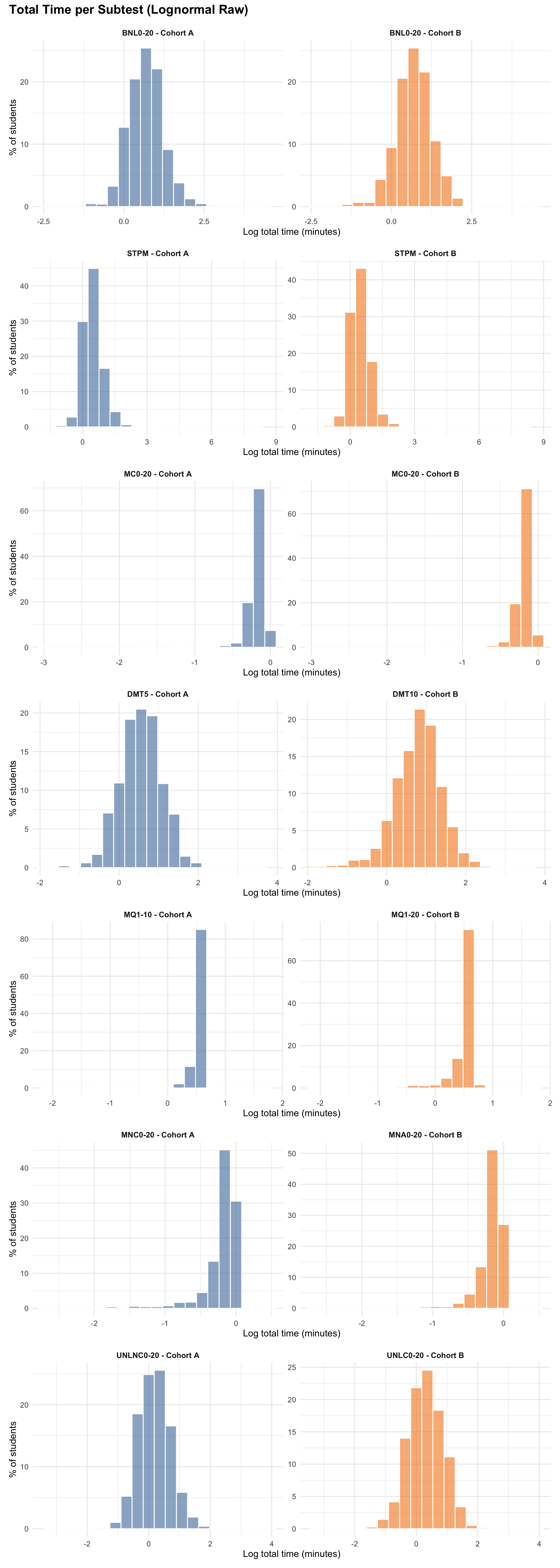
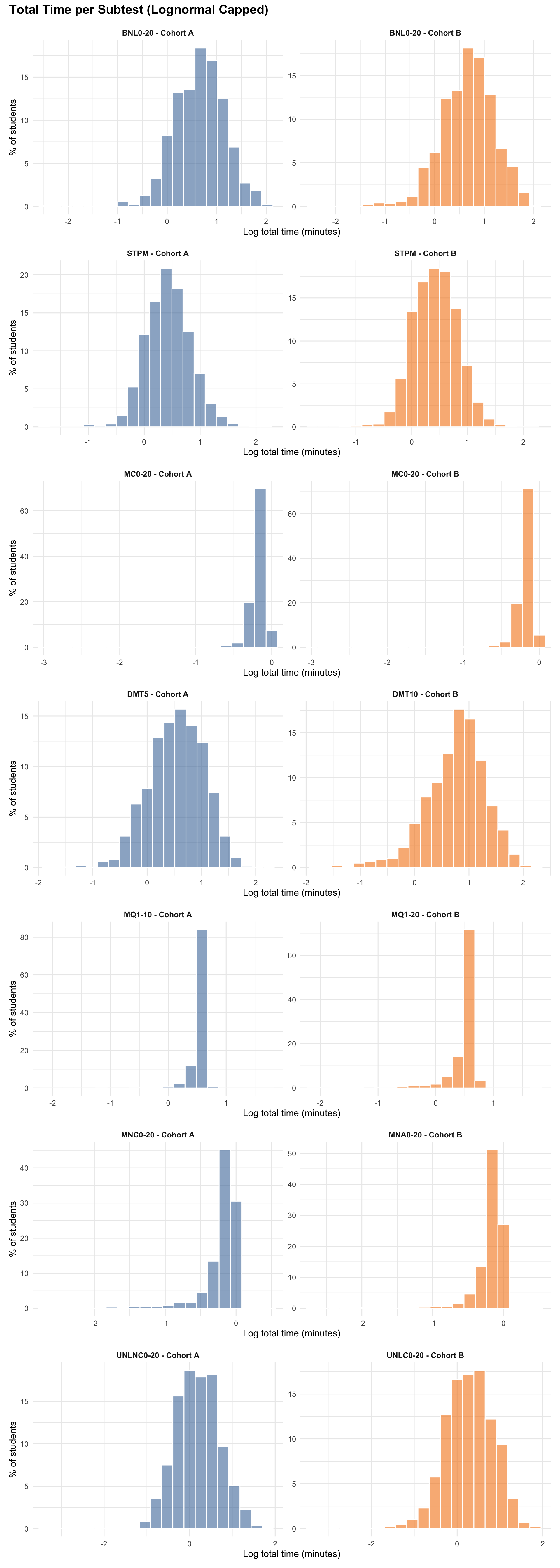
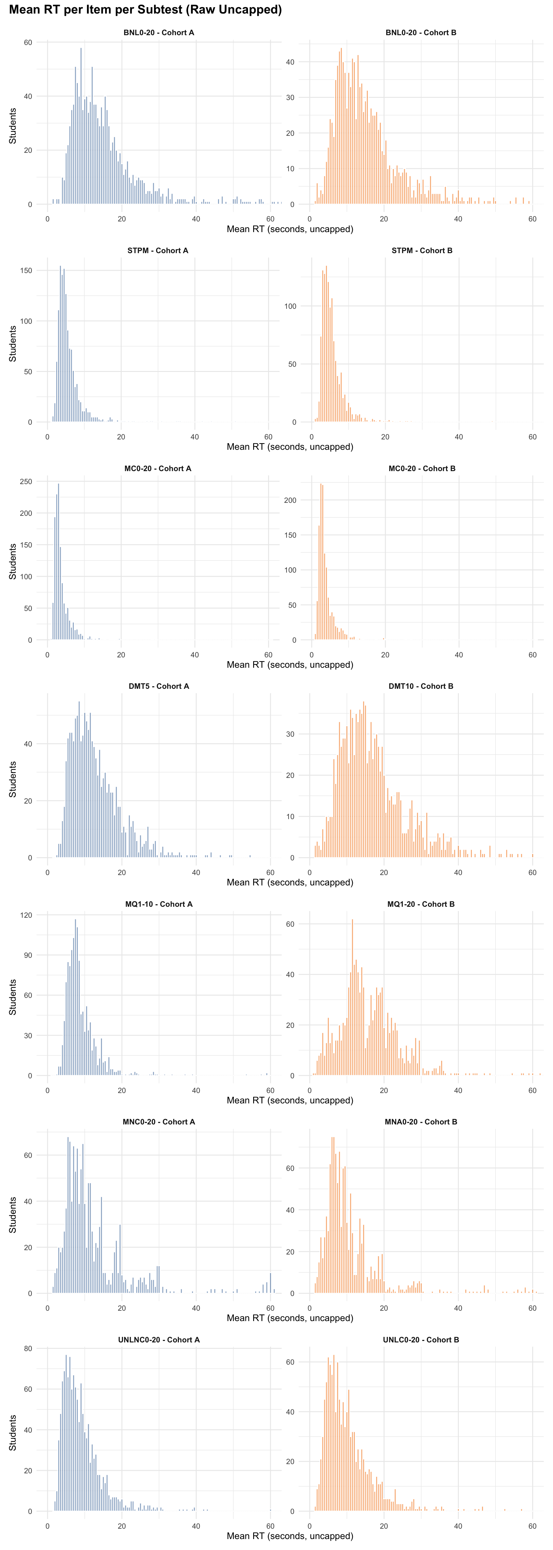
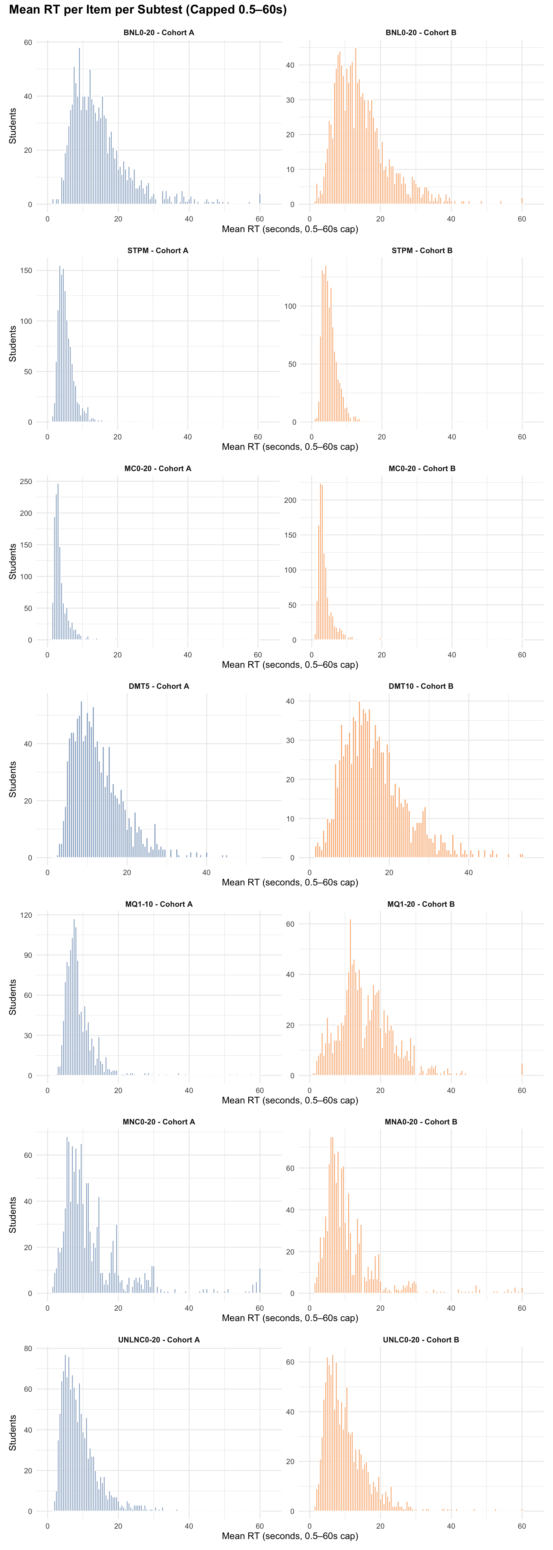
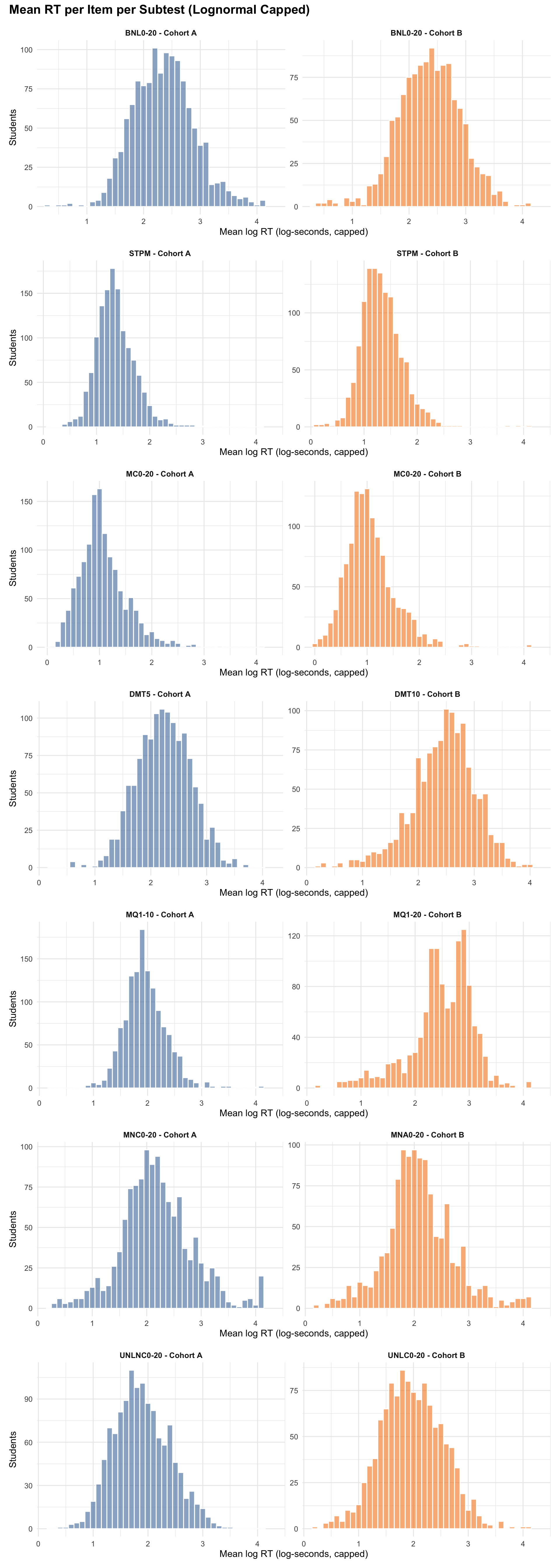
- EDA summaries: Response times are capped at 0.5–60 seconds for per-response summaries in this exploratory data analysis section to provide robust descriptive statistics.
- Model preprocessing: Timed items use a 0.5–60 second cap, while untimed items use a 0.5–180 second cap (sensitivity runs only; baseline model excludes untimed RTs).
- Rationale: Prevents very long untimed RTs from dominating model estimation while allowing exploratory analysis of untimed response patterns.
3.1 RT Distributions
3.1.1 Total Response Time (per student)
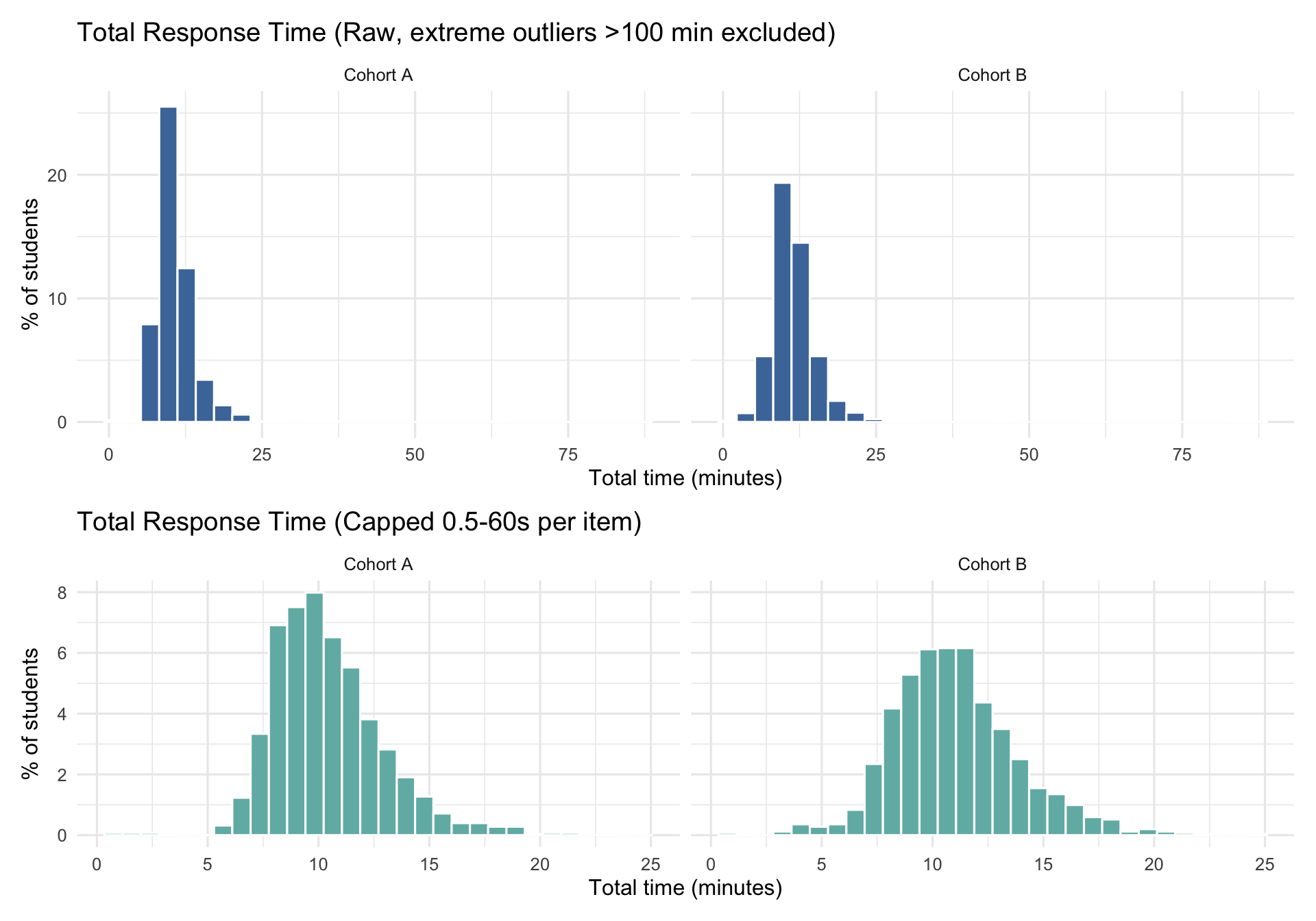
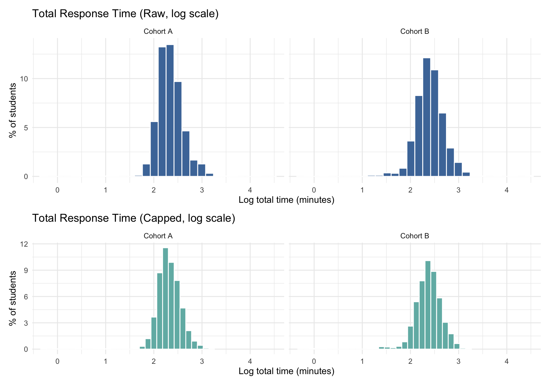
3.1.2 Total Time by Subtest (per student)
3.2 Item-Level RT Diagnostics
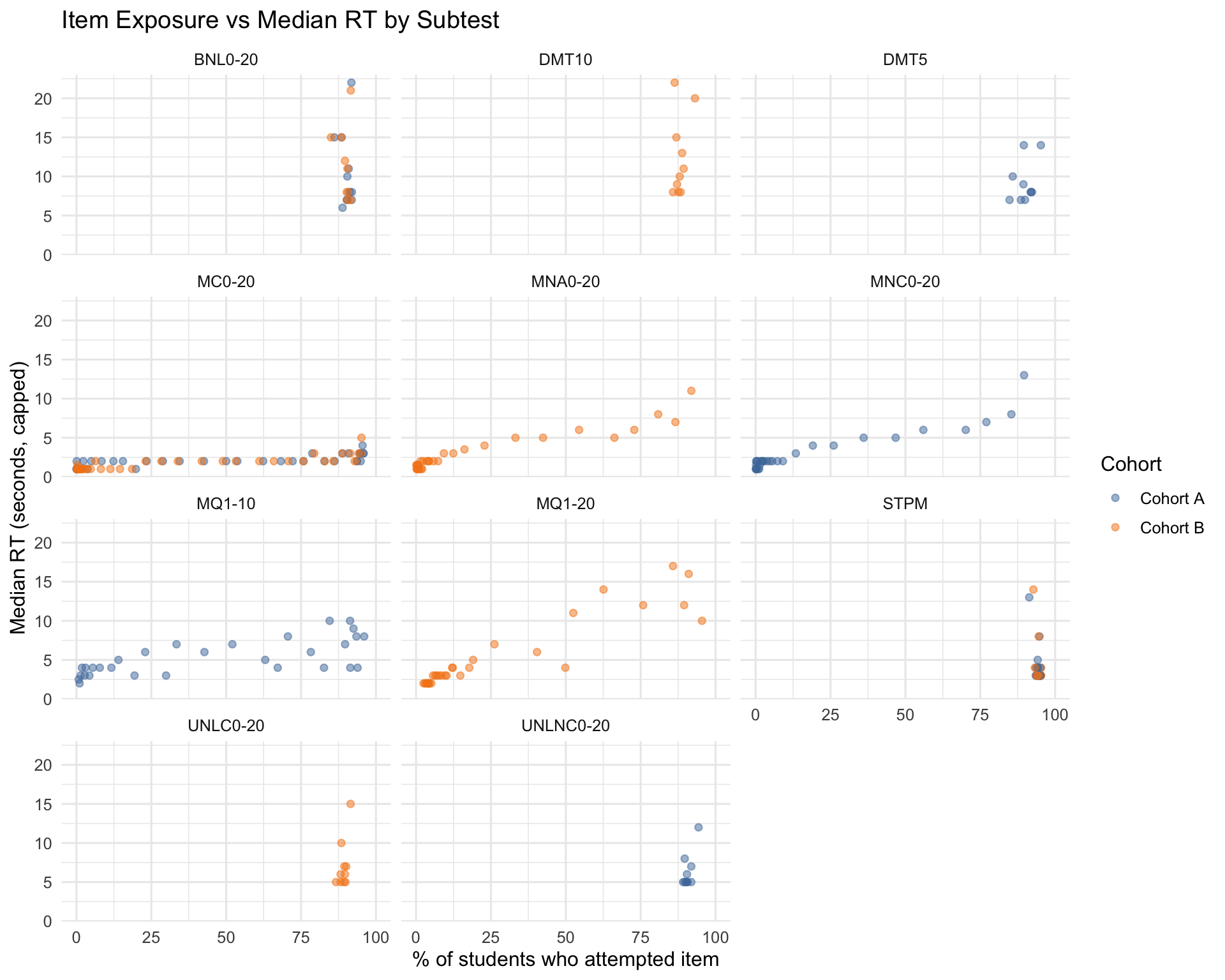
This plot shows the relationship between what percentage of students in each cohort attempted each item (x-axis) and the median response time (y-axis). Items with very low exposure (near 0%) may have unreliable RT estimates. Items with unusually high or low RT compared to peers in the same subtest warrant investigation for clarity or technical issues.
3.2.1 RT Deltas: Incorrect vs Correct (Timed vs Untimed)
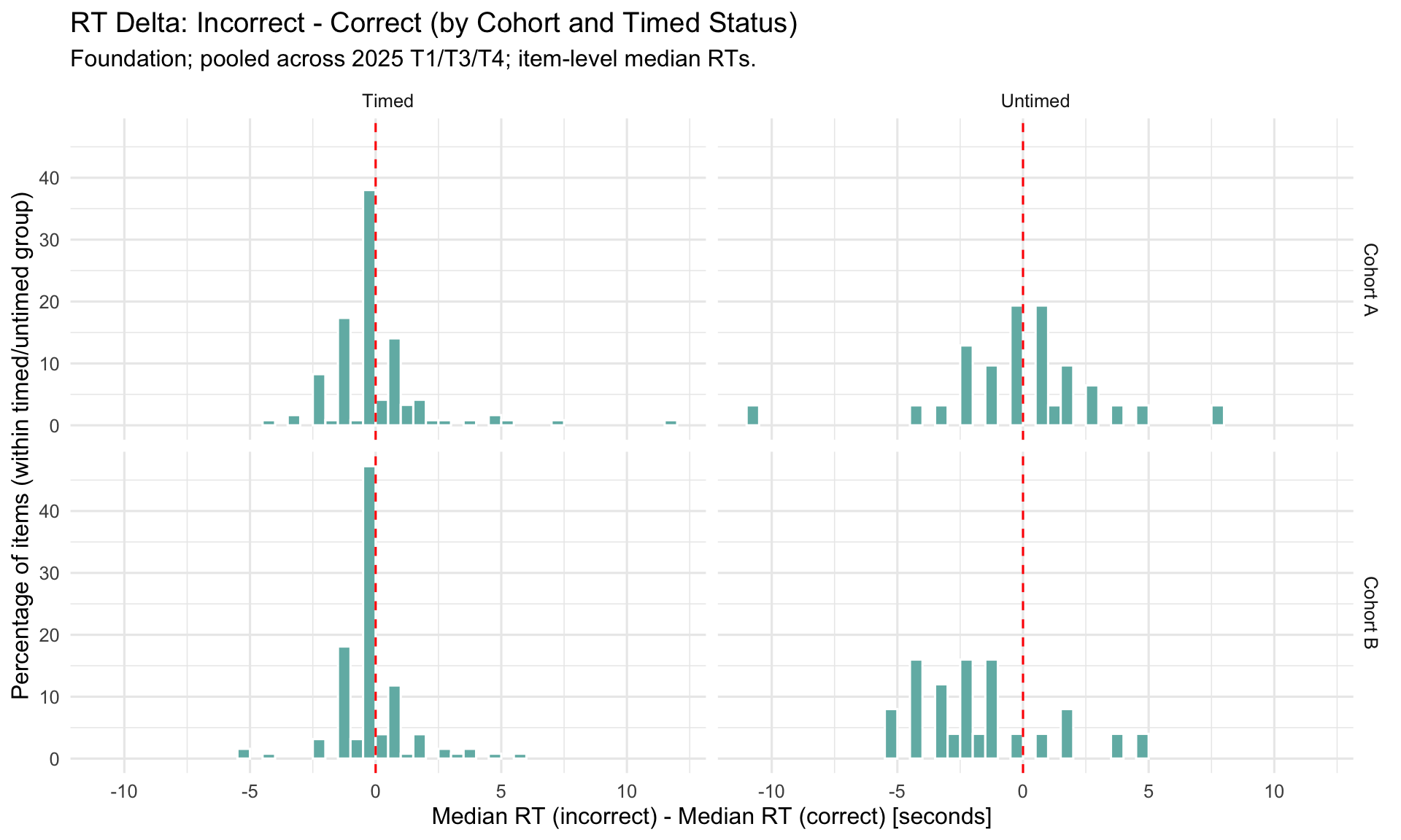
Pooled across 2025 terms (T1/T3/T4).
3.2.2 Correct vs Incorrect RT (Timed Math) by Subtest
The relationship between response time (RT) and correctness is probe-dependent.
3.2.3 Diagnosing fast-wrong responses
Rapid responses (defined as ≤ 1 second) paired with incorrect answers can indicate rapid guessing or UI/technical issues. These can inflate estimated speed by adding very short response times that are unlikely to reflect genuine fluent responding.
We computed subtest-level fast–wrong and fast–correct rates for timed, non-speed-test maths subtests (within Term 1 × cohort × subtest) and pooled counts by subtest (response-weighted), reporting fast–wrong excess (fast–wrong minus fast–correct) as the primary diagnostic. Results indicate subtest-dependent response behaviour, consistent with differences in item format or interaction demands.
In this v3 run, the RT likelihood uses all timed RTs; these diagnostics are intended to inform a probe-aware RT inclusion policy for the next iteration (e.g., model correct-only RT for probes with high fast-wrong rates and large fast-wrong excess).
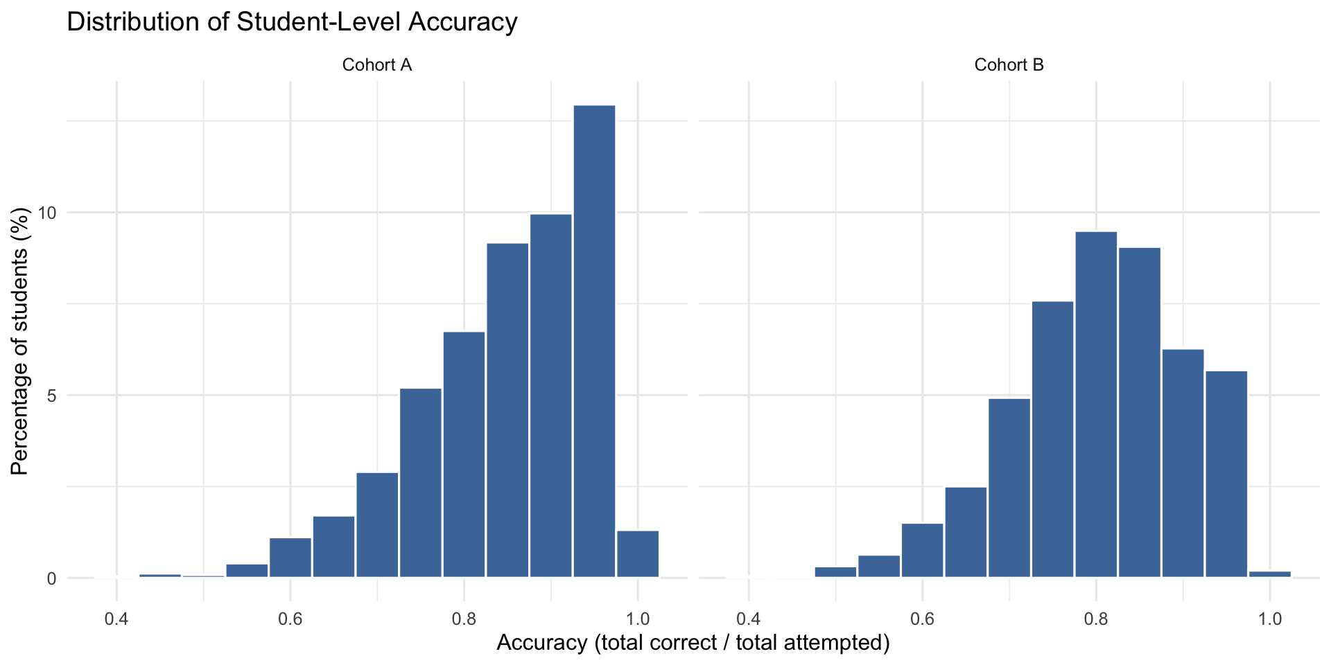
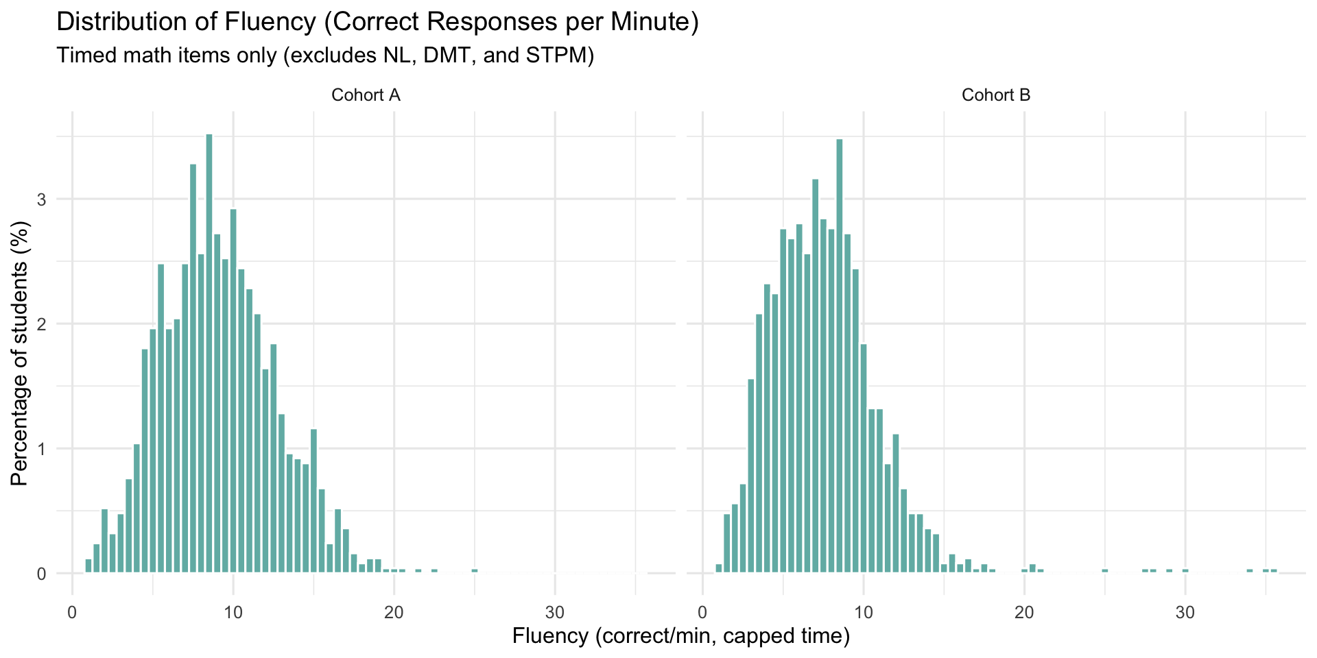
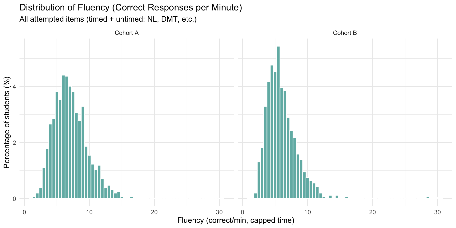
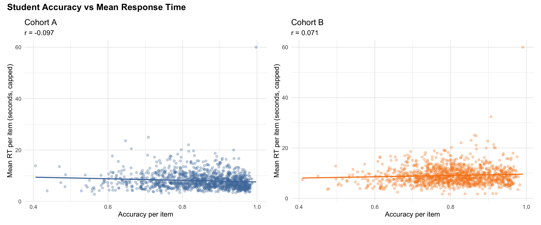
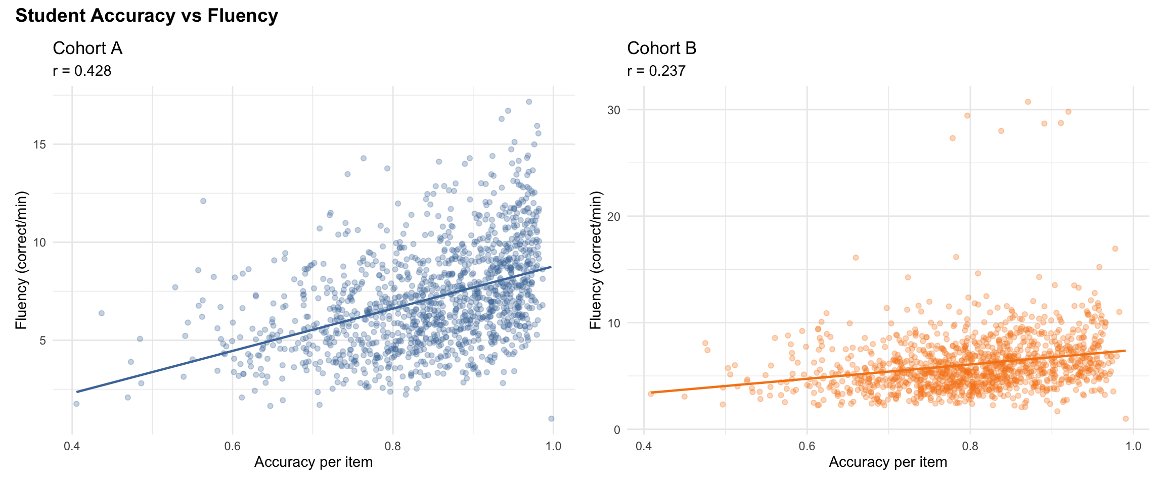
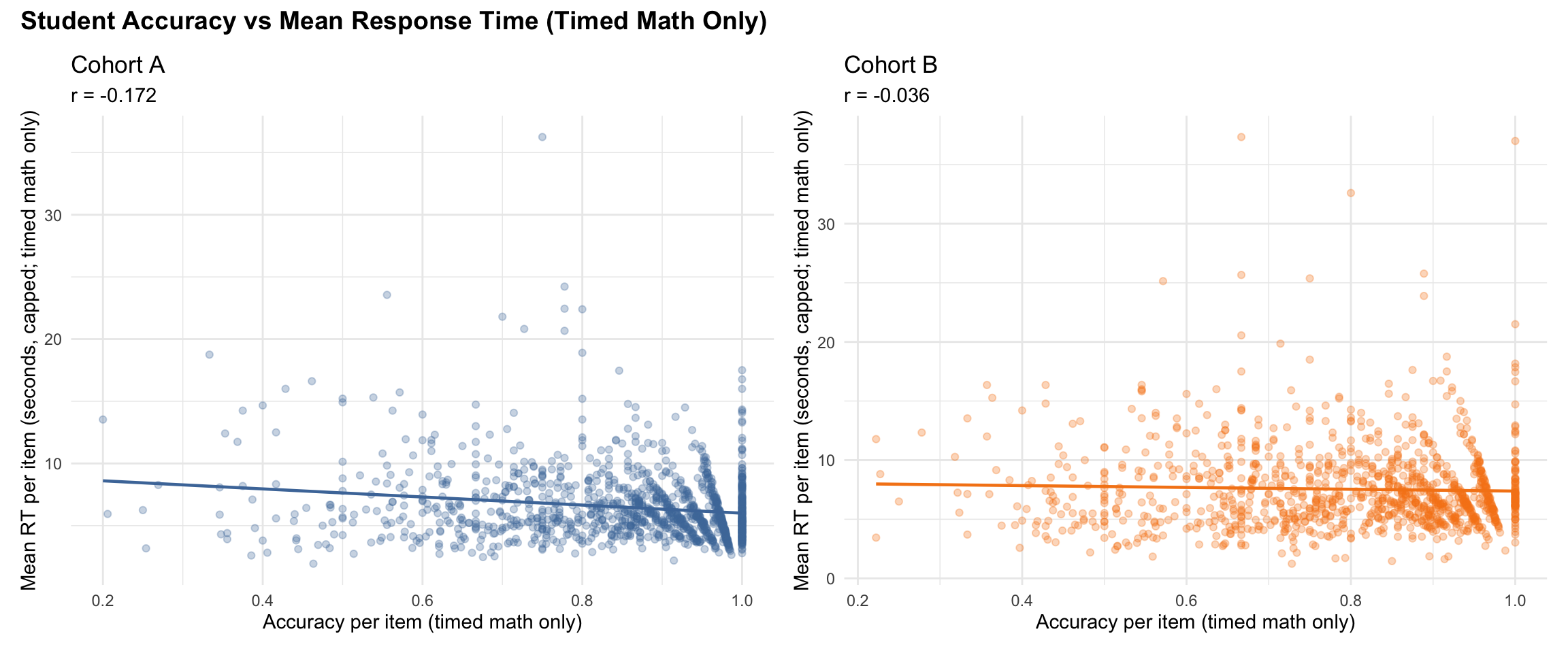
4 Student Performance (Model-Free)
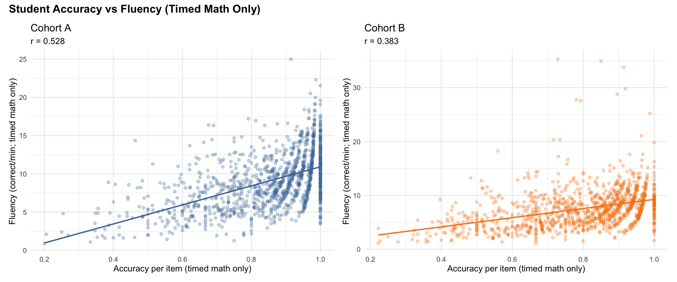
5 Subtest Results
| test_subgroup | exam_group_cohort | n_students | median_items | median_time_min | median_accuracy | median_fluency |
|---|---|---|---|---|---|---|
| BNL0-20 | F-A | 1290 | 10 | 1.98 | 0.86 | 3.81 |
| BNL0-20 | F-B | 1196 | 10 | 2.03 | 0.86 | 3.73 |
| DMT10 | F-B | 1197 | 10 | 2.27 | 0.30 | 1.26 |
| DMT5 | F-A | 1288 | 10 | 1.74 | 0.61 | 2.82 |
| MC0-20 | F-A | 1289 | 16 | 0.83 | 0.93 | 17.50 |
| MC0-20 | F-B | 1197 | 16 | 0.83 | 0.92 | 16.80 |
| MNA0-20 | F-B | 1172 | 6 | 0.88 | 0.83 | 5.66 |
| MNC0-20 | F-A | 1245 | 5 | 0.88 | 0.83 | 4.29 |
| MQ1-10 | F-A | 1288 | 14 | 1.80 | 0.96 | 7.07 |
| MQ1-20 | F-B | 1201 | 7 | 1.78 | 0.78 | 3.13 |
| STPM | F-A | 1295 | 20 | 1.53 | 1.00 | 12.39 |
| STPM | F-B | 1209 | 20 | 1.52 | 1.00 | 12.39 |
| UNLC0-20 | F-B | 1178 | 10 | 1.33 | 0.81 | 5.50 |
| UNLNC0-20 | F-A | 1280 | 10 | 1.20 | 0.81 | 6.14 |
5.0.1 Items Attempted per Subtest
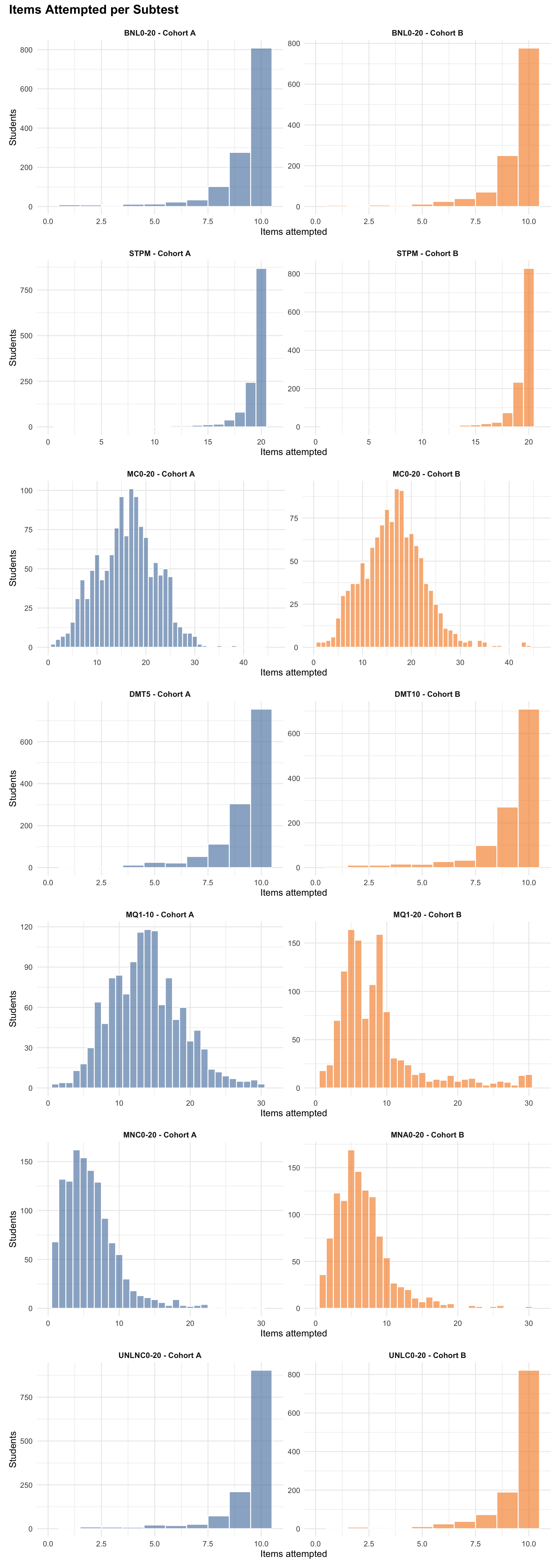
5.0.2 Total Time per Subtest
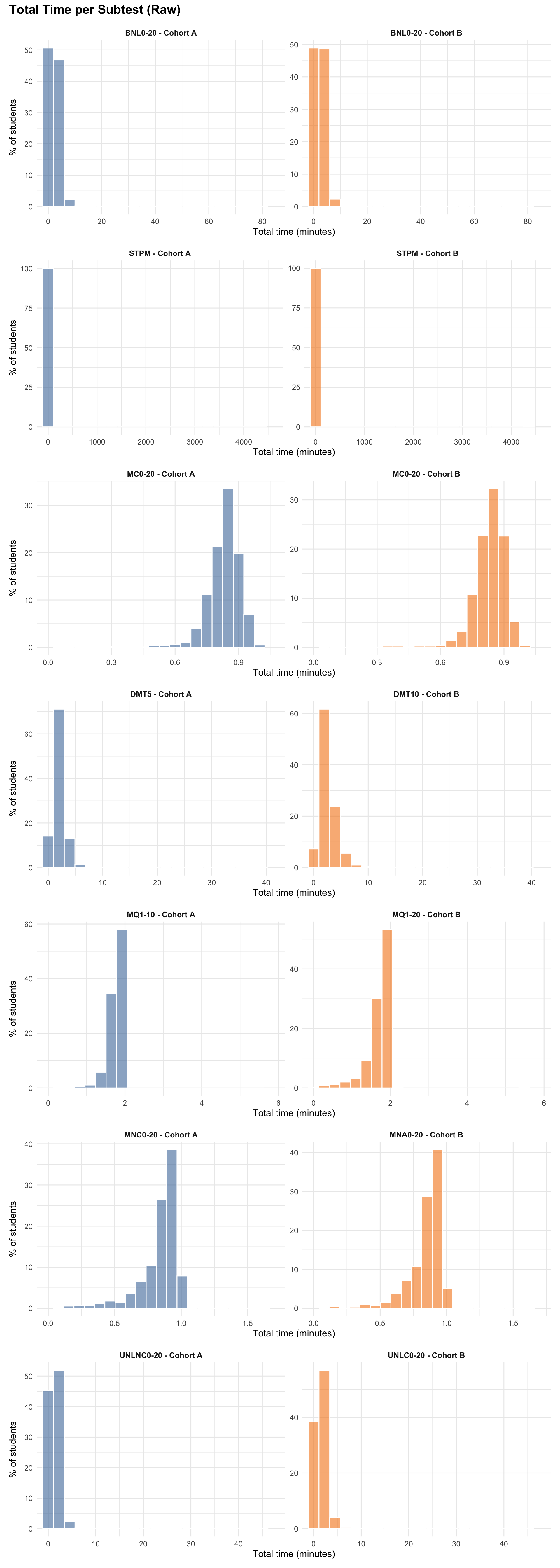
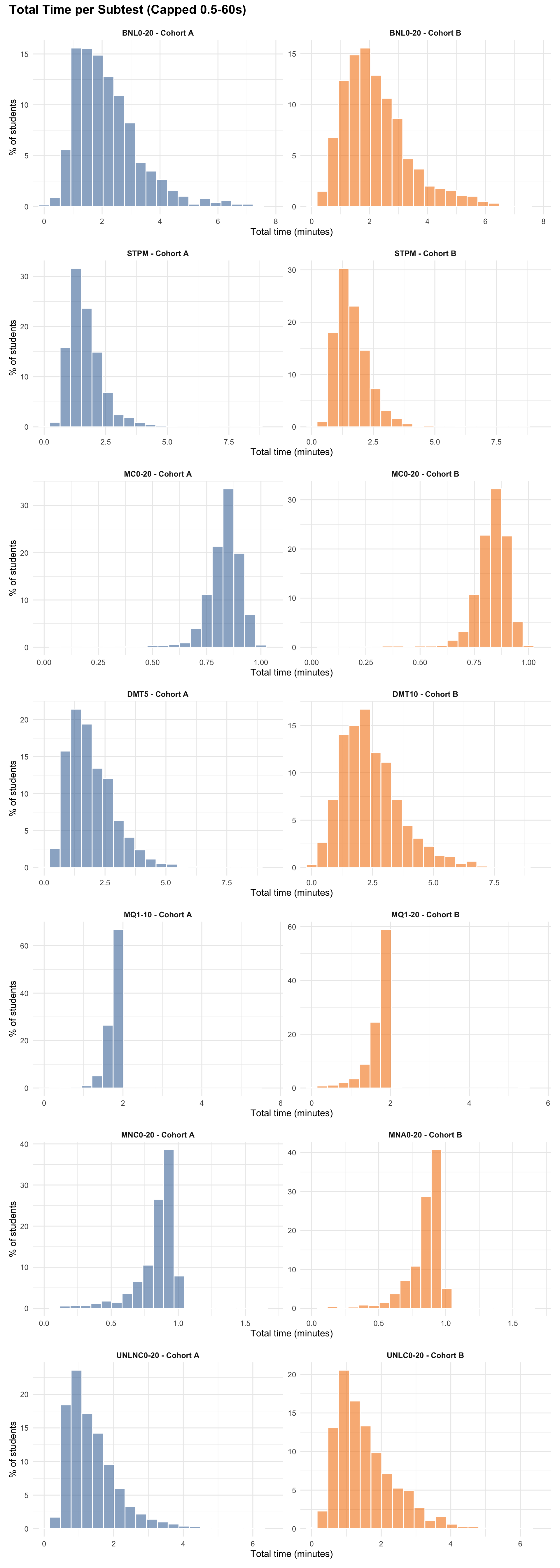
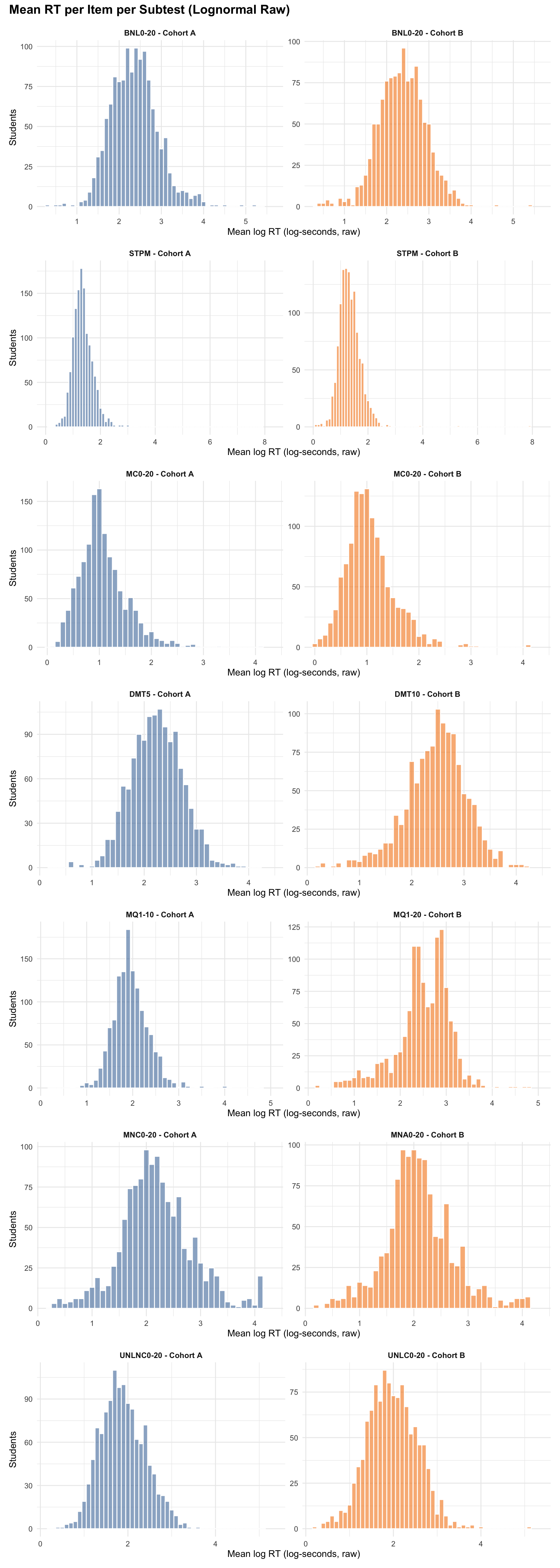
5.0.3 Mean RT per Item per Subtest
6 IRT Model Overview
The joint model estimates accuracy and timed responding as separate but correlated latent traits, and produces a derived residual for analytic work.
6.1 What the model estimates
| Construct | Description | Interpretation |
|---|---|---|
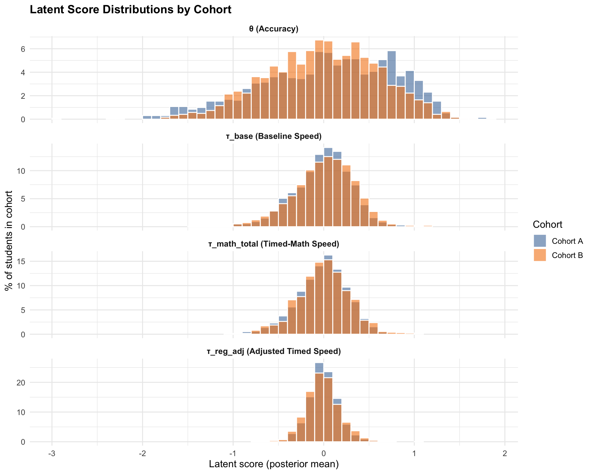
| θ (theta) | Accuracy on numeracy items | Higher = more accurate |
| τ_base | Baseline timed responding speed anchored by STPM | Higher = faster (lower RT) |
| τ_math_total | Absolute timed-math speed (headline fluency) | Higher = faster (lower RT) |
| τ_reg_adj | Regression-adjusted timed-math speed (residual after accounting for τ_base) | Higher = faster than expected given baseline speed |
RT is modelled on the log scale as log(RT) = lambda_item - tau_person + noise.
- Higher tau = faster.
- A 0.3 increase in tau corresponds to roughly
exp(-0.3) ≈ 0.74×RT (about 25% faster), holding item time-intensity constant.
To align with common conventions, speed will be denoted with zeta rather than tau in future updates. Tau is typically reserved for partial credit model step parameters.
6.1.1 Response coding
Binary items (0/1)
Binary items (MC, MNA, MNC, MQ, DMT) use a Rasch (1PL) model with difficulty parameter b (discrimination fixed to 1).
Number-line items (3-category PCM)
NL items record continuous accuracy (0–1) and are discretised into 3 ordered categories:
- Category 0:
raw_score < 0.80 - Category 1:
0.80 ≤ raw_score < 0.95 - Category 2:
raw_score ≥ 0.95
These are modelled using a partial credit model (PCM) with difficulty b and two step thresholds (step₁, step₂).
6.1.2 RT preprocessing
Timed RTs are preprocessed with:
- Floor: 0.5 seconds
- Cap: 60 seconds for timed items
- Transformation:
log(rt_adj) - Untimed items: Excluded from the RT likelihood entirely. Sensitivity runs used a 0.5–180 second cap; the baseline model uses no untimed RTs.
Only STPM (baseline) and timed math items contribute to the RT likelihood.
6.2 Model structure
6.2.1 Accuracy component (Rasch + PCM)
Binary items: \[P(Y_{ij} = 1 | \theta_i, b_j) = \text{logit}^{-1}(\theta_i - b_j)\]
Parameters:
- \(Y_{ij}\): response for student \(i\) on item \(j\) (1 = correct, 0 = incorrect)
- \(\theta_i\): accuracy trait for student \(i\)
- \(b_j\): difficulty for item \(j\)
NL items (PCM): \[P(Y_{ij} = k | \theta_i, b_j, \text{step}_{j,\cdot}) \propto \exp\left(\sum_{c=1}^k (\theta_i - b_j - \text{step}_{j,c})\right)\]
Parameters:
- \(Y_{ij}\): ordered category for student \(i\) on item \(j\) (0, 1, 2)
- \(k\): category index
- \(b_j\): difficulty for item \(j\)
- \(\text{step}_{j,c}\): step threshold \(c\) for item \(j\)
6.2.2 Response-time component
For each RT observation:
\[\log(RT_{ij}) \sim \text{Normal}(\lambda_j - \tau_{eff,i}, \sigma_{rt,g})\]
Parameters:
- \(RT_{ij}\): response time for student \(i\) on item \(j\) (seconds)
- \(\lambda_j\): item time-intensity parameter
- \(\tau_{eff,i}\): effective speed for student \(i\) on item \(j\)
- \(\sigma_{rt,g}\): RT noise SD for subgroup \(g\)
- \(g\): RT subgroup (speed anchor vs timed math)
where:
- \(\tau_{eff,i} = \tau_{base,i}\) for STPM anchor items
- \(\tau_{eff,i} = \tau_{math\_total,i}\) for timed math items
6.2.3 Correlation structure
Latent traits are jointly modelled with a multivariate normal correlation structure on a standardised latent vector. Cohort linking for θ uses group-specific mean/SD (Cohort A fixed to 0/1).
6.2.4 Priors (summary)
| Parameter | Prior | Role |
|---|---|---|
z_person |
Normal(0, 1) | Non-centred latent factors (θ_z, τ_math, τ_base) |
L_corr |
LKJ(2) | Cholesky factor of 3×3 latent correlation matrix |
sigma_tau |
Normal⁺(0, 1) | Speed component SDs [2]: math, baseline |
theta_mu_free |
Normal(0, 1) | Cohort mean accuracy (Cohort A fixed to 0) |
theta_sd_free |
Normal⁺(1, 0.5) | Cohort SD accuracy (Cohort A fixed to 1) |
b |
Normal(0, 1.5) | Item difficulty |
step_raw |
Normal(0, 1.5) | PCM step parameters (mean-centred within item) |
lambda |
Normal(0, 1.0) | Item time-intensity |
sigma_rt |
Normal⁺(0, 0.5) | RT residual SD per subgroup |
Normal⁺ denotes a half-normal prior (parameter declared with <lower=0> in Stan). The model uses a non-centred parameterisation: raw latent factors z_person are standard normal, then scaled by diag(sigma_trait) * L_corr to obtain correlated (θ_z, τ_math, τ_base). Cohort A is anchored at mean = 0, SD = 1 for θ; Cohort B’s mean and SD are estimated freely. Step parameters are mean-centred within each item; step ordering is checked post-fit but not enforced during sampling.
7 Model Results
This section reports latent scores for Foundation students. For operational use, the recommended pair is θ (accuracy) and τ_math_total (timed-math speed). Use τ_base as contextual baseline speed and treat τ_reg_adj as an analytic residual rather than the headline speed score.
7.1 Latent Score Distributions
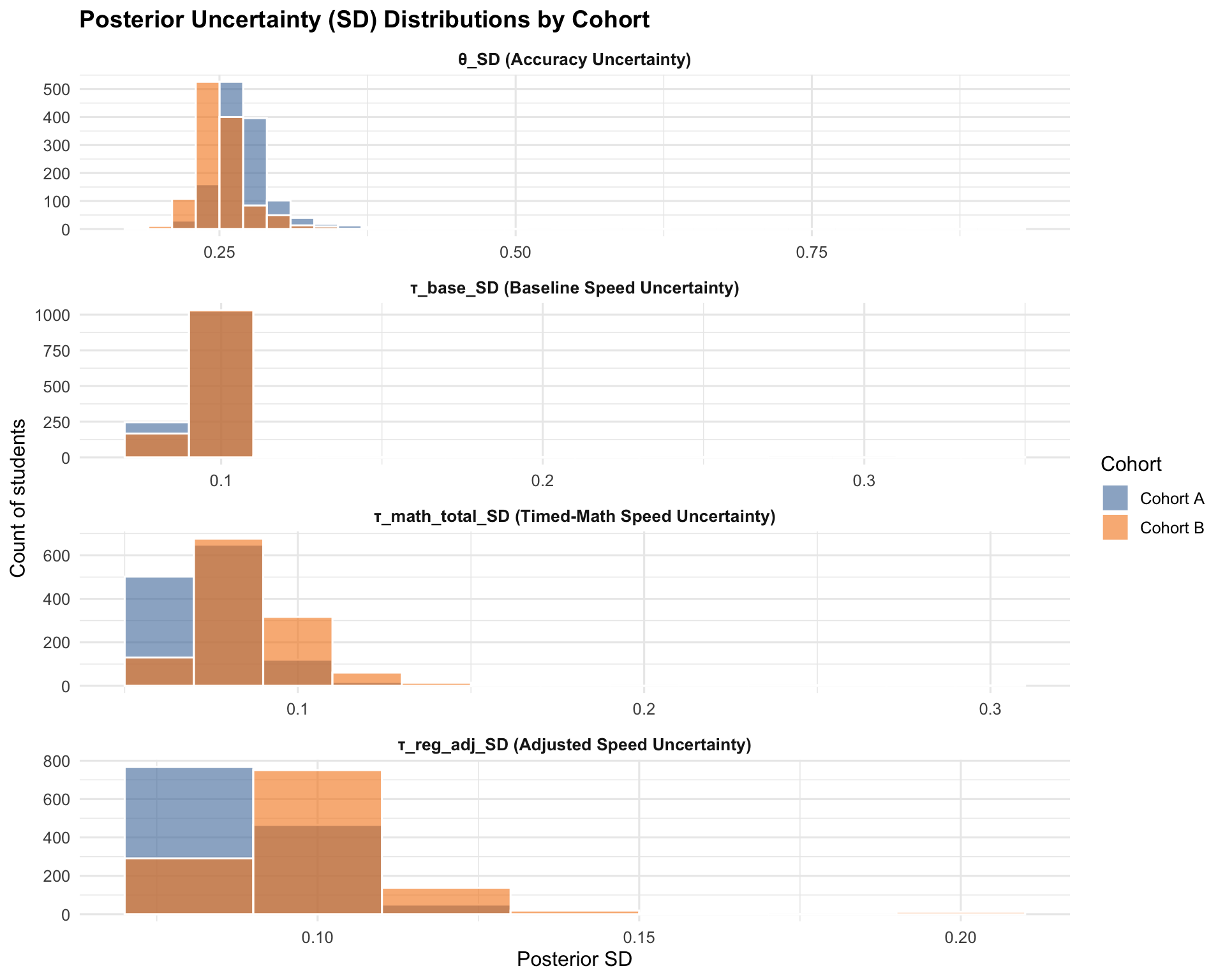
7.2 Uncertainty Distributions
7.3 Scale precision and reliability
Posterior SDs provide a conditional SEM-style view of precision along the θ scale. The plot below bins students by θ and summarizes uncertainty within each bin.
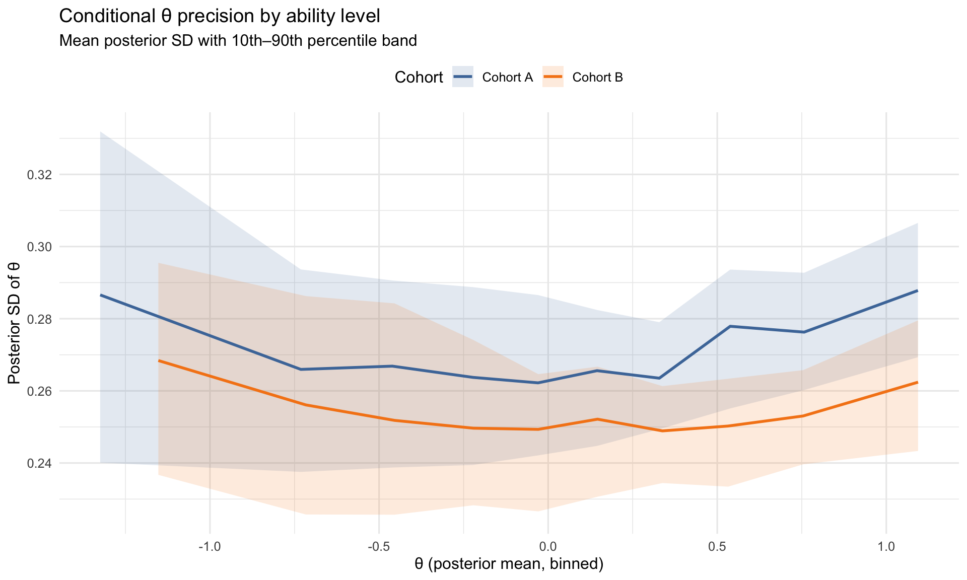
| Cohort | var_theta | mean_se2 | marginal_reliability |
|---|---|---|---|
| Cohort A | 0.554 | 0.076 | 0.880 |
| Cohort B | 0.377 | 0.065 | 0.853 |
7.4 Construct checks (latent vs observed)
These checks verify that latent scores align with direct, model-free summaries from the raw data.
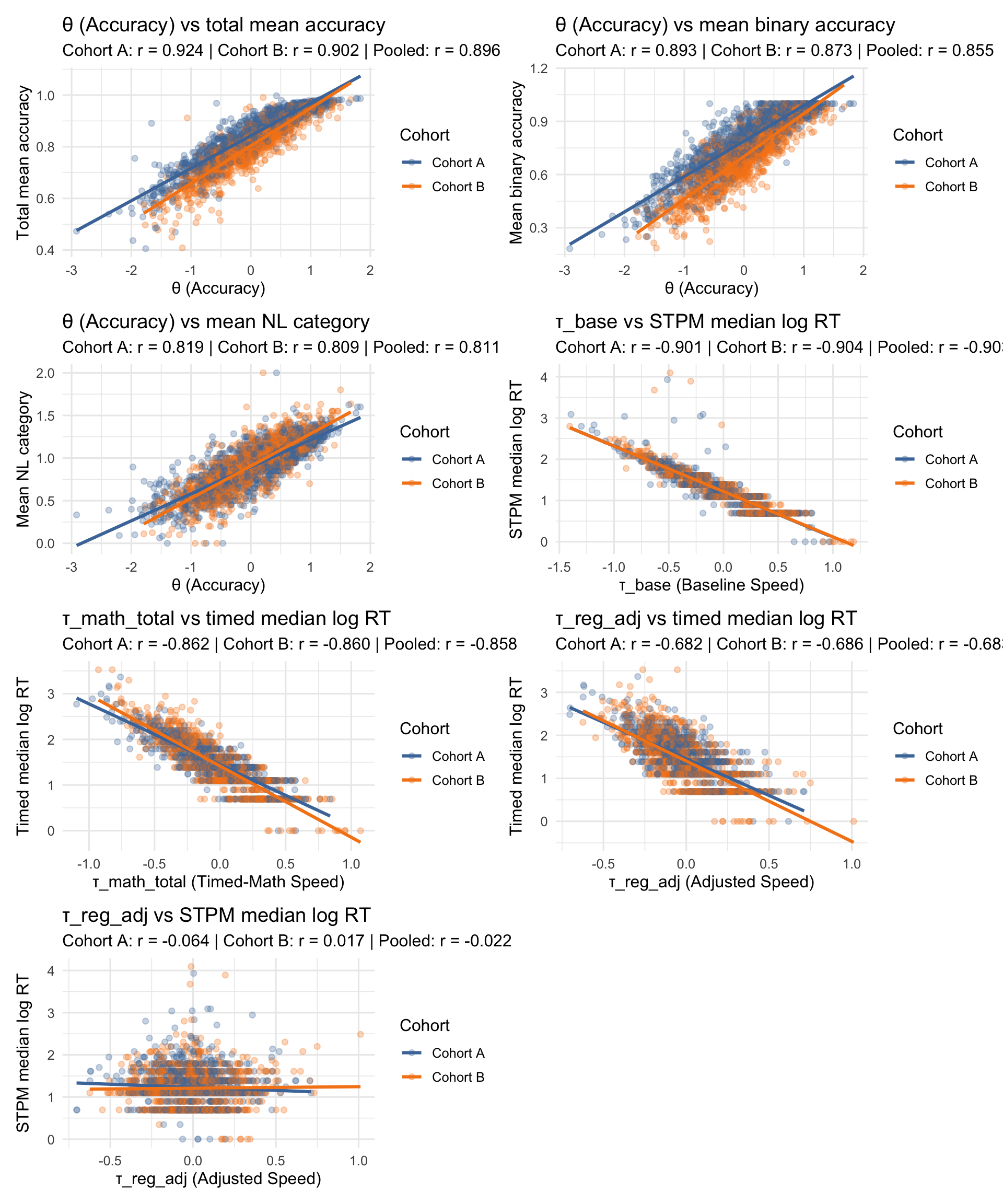
The expected patterns appear: θ tracks accuracy, τ_base tracks STPM speed, τ_math_total tracks timed-math speed, and τ_reg_adj is largely independent of baseline speed.
7.5 Correlation plots (latent scores)
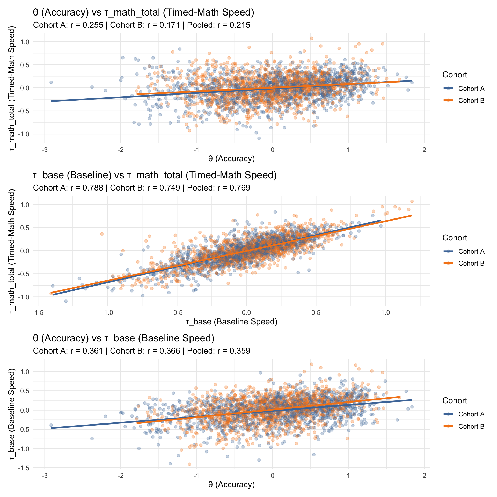
The three panels show the expected construct pattern. θ vs τ_math_total (pooled r = 0.22) shows a positive correlation — more accurate students tend to respond faster on timed math items. τ_base vs τ_math_total (pooled r = 0.77) shows a strong positive correlation, confirming a general speed factor: students fast on baseline pattern matching are also fast on timed math. θ vs τ_base (pooled r = 0.36) shows a weaker relationship, indicating that accuracy is largely separable from baseline motor speed — supporting discriminant validity of the accuracy construct.
7.6 Low-Information Flagging Rates
Students are flagged as low-information when they have too few responses or unusually wide posterior uncertainty:
- Low accuracy items:
n_acc_total < 20 - Low timed-math RT count:
n_timed_math_rt < 10 - Low STPM RT count:
n_speed_rt < 10 - Low θ precision:
theta_sd > 0.7 - Low τ_reg_adj precision:
tau_reg_adj_sd > 0.7 - Low info (any): flagged on any of the above
High rates indicate thin data, not necessarily poor model fit. Thresholds are configurable in the model pipeline; defaults are shown here.
| exam_group_cohort | n_students | n_low_acc_items | n_low_timed_math_rt | n_low_speed_rt | n_low_theta_precision | n_low_tau_reg_precision | n_low_info_any | pct_low_acc_items | pct_low_timed_math_rt | pct_low_speed_rt | pct_low_theta_precision | pct_low_tau_reg_precision | pct_low_info_any |
|---|---|---|---|---|---|---|---|---|---|---|---|---|---|
| F-A | 1302 | 10 | 18 | 18 | 2 | 0 | 29 | 0.8 | 1.4 | 1.4 | 0.2 | 0 | 2.2 |
| F-B | 1215 | 14 | 30 | 10 | 0 | 0 | 32 | 1.2 | 2.5 | 0.8 | 0.0 | 0 | 2.6 |
7.7 Prior Predictive Checks
The prior predictive check verifies that the model’s priors are weakly informative — they should generate plausible data without concentrating on pathological regions of the parameter space. We simulate from the prior distributions using pure R (no Stan refit), drawing synthetic students and items to check the implied ranges.
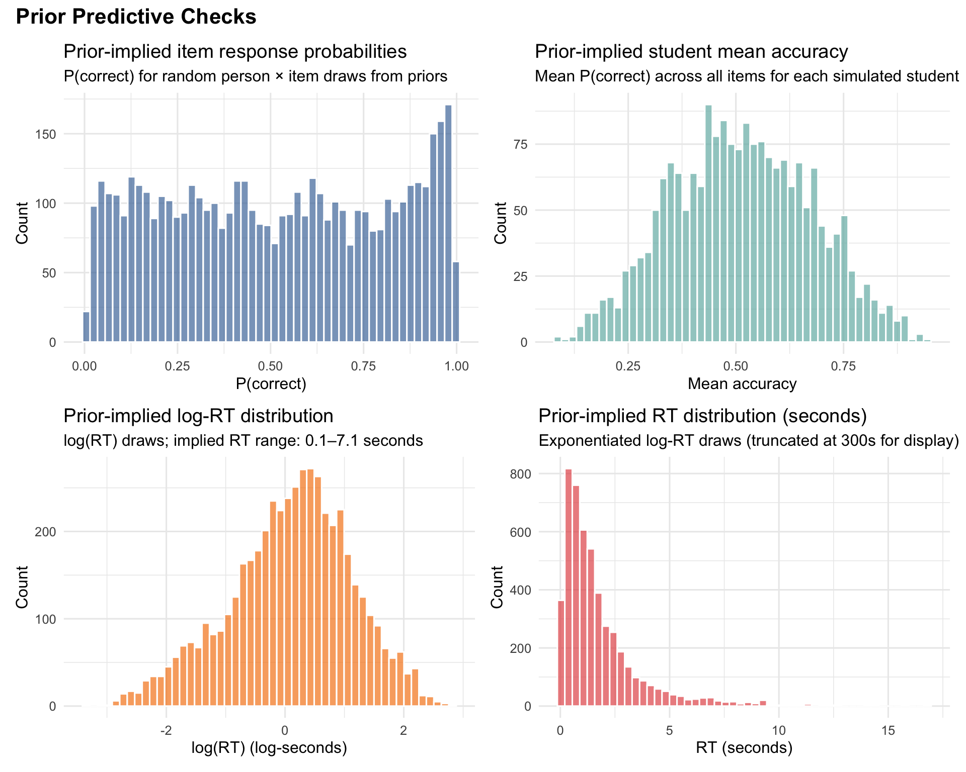
The prior predictive distributions cover sensible ranges without pathological concentration. Item response probabilities span the full 0–1 range, student mean accuracies centre near 0.5 with reasonable spread, and prior-implied RTs cover the plausible range of observed response times. The priors are weakly informative — they express mild expectations about parameter scale without constraining the posterior to a narrow region.
7.8 Posterior Predictive Checks
For each of 200 posterior draws (subsampled from the full MCMC output), we simulate replicated data from the fitted model and compare summaries of replicated data to the observed data. This is the standard Bayesian posterior predictive check (Gelman et al., 2013).
- Grey lines/bars show what the fitted model predicts across replicated datasets (90% posterior predictive interval).
- Dots/blue curves show the observed data.
- If the observed statistic falls outside the predictive interval, the model does not reproduce that feature of the data (or the PPC computation needs auditing). A few misses are expected when many checks are run; systematic misses are the main concern.
7.8.1 Total score distribution
7.8.2 Item calibration
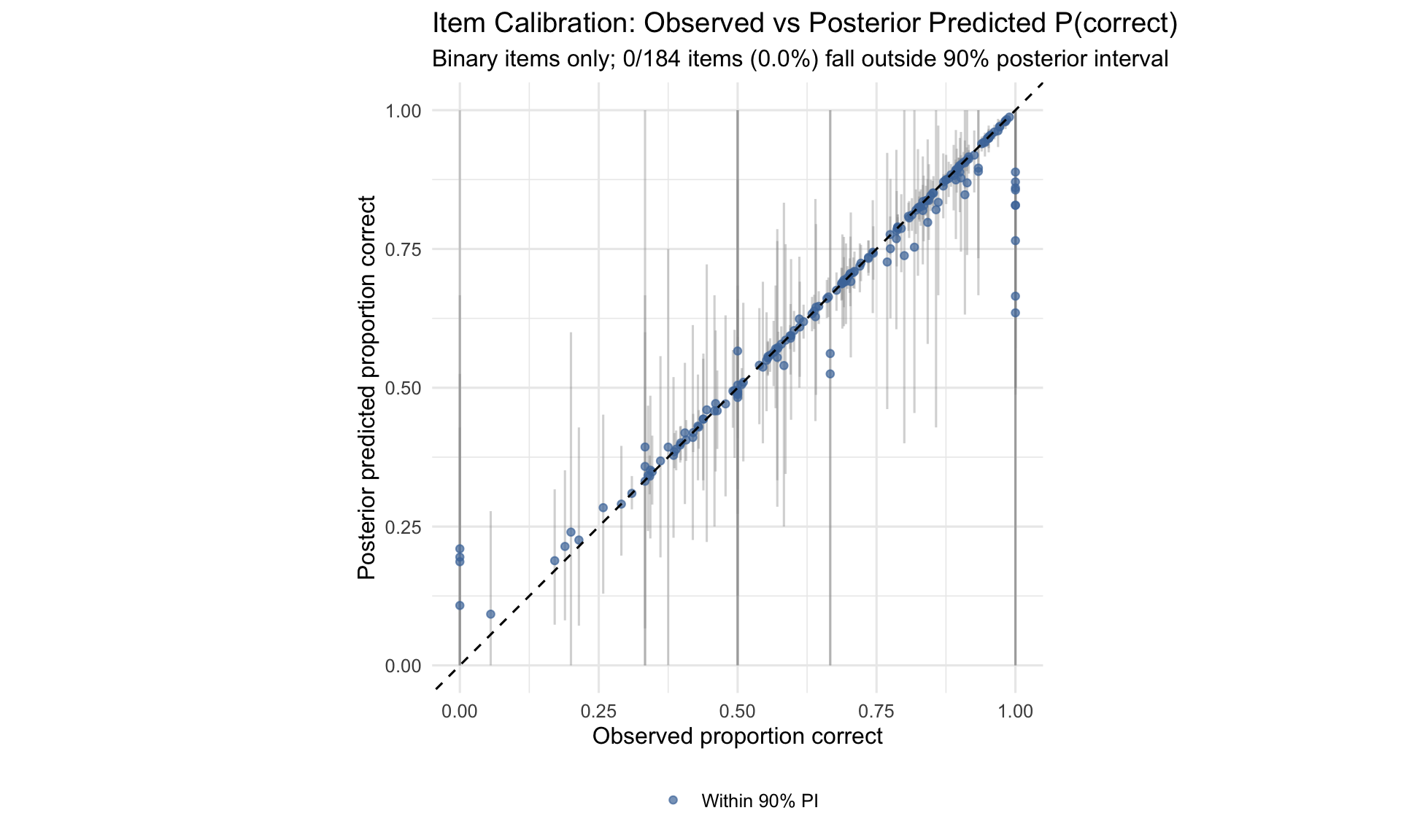
7.8.3 Summary statistics
| Statistic | Observed | Posterior mean | 90% PI lower | 90% PI upper |
|---|---|---|---|---|
| Mean total score | 49.03 | 49.00 | 48.82 | 49.19 |
| SD total score | 17.55 | 17.62 | 17.46 | 17.79 |
The posterior predictive checks compare observed summaries to summaries computed on replicated datasets drawn from the fitted model’s posterior. The total score density overlay is a global shape check (replicated distributions in grey vs observed in blue). The item calibration plot is an in-sample internal consistency check for binary items: it asks whether the model recovers each item’s observed proportion-correct within posterior uncertainty.
The mean/SD table is a coarse diagnostic. If the observed mean/SD fall outside the predictive interval, first audit that the observed and replicated scores use identical inclusion rules and scoring (NL discretisation/indexing is a common source of PPC mismatch); persistent shifts then suggest mild global misfit rather than item-specific problems.
7.8.4 RT component checks
These checks compare observed log-RT summaries against posterior predictive replicates for the RT likelihood (STPM + timed math). Log-RT summaries are computed on the same floored/capped scale used for model fitting.
Subtest log-RT quantiles
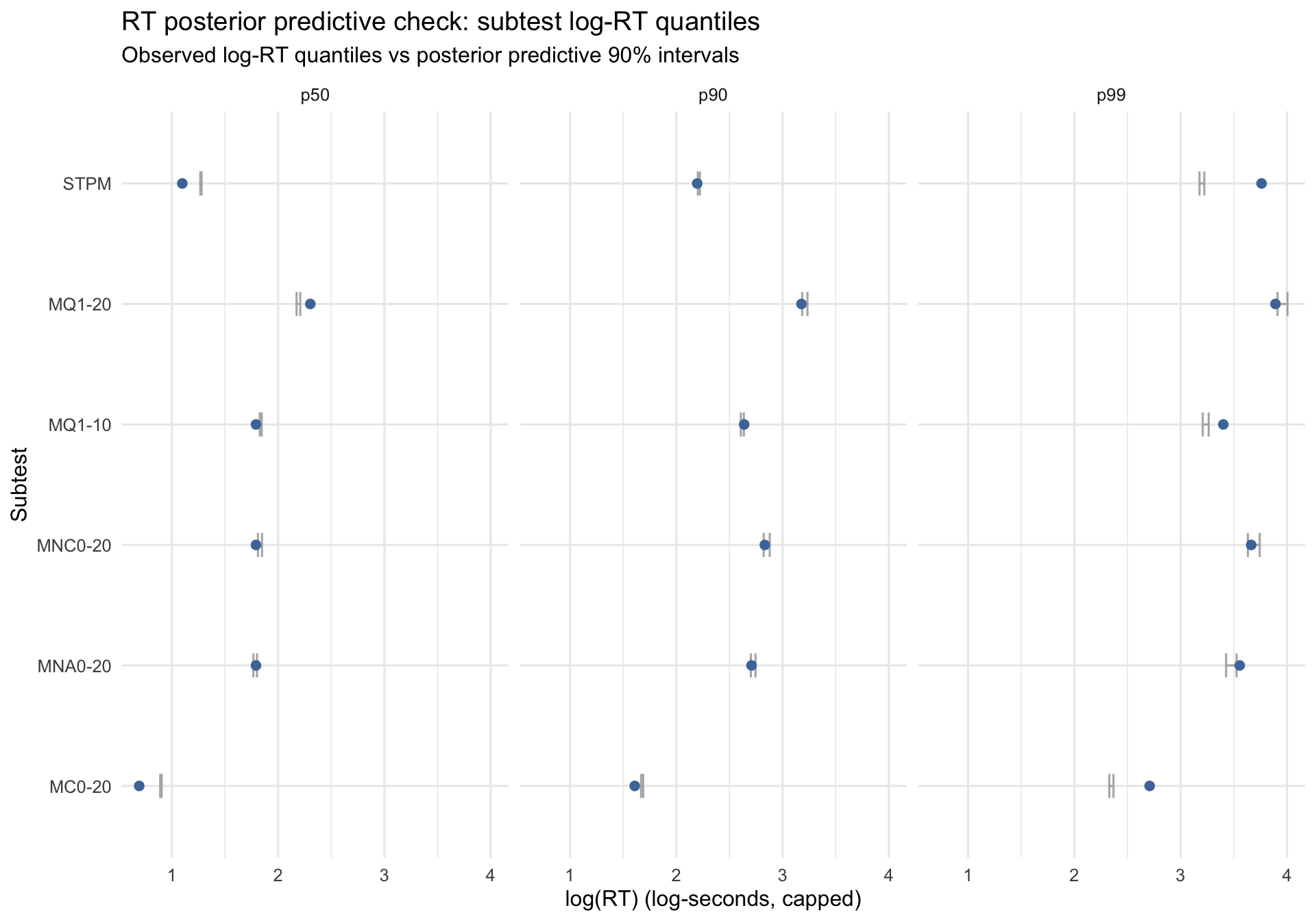
Interpretation: p50 reflects the typical (median) response time within each subtest; p90 and p99 focus on the slow tail (including pauses). Dots outside the grey interval indicate the fitted RT model does not reproduce that part of the distribution. Interval width varies with the number of RT observations and posterior uncertainty.
RT cap rate by subtest
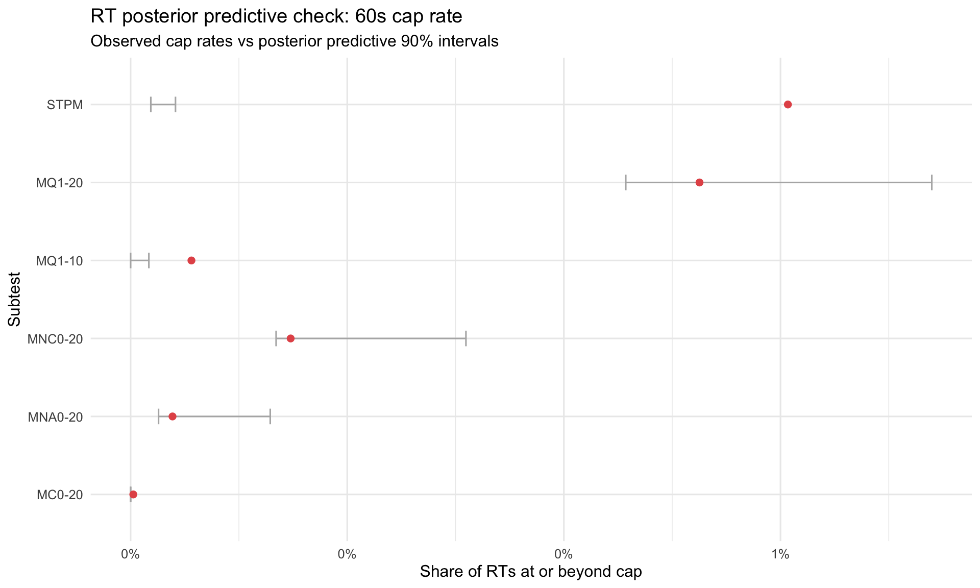
Interpretation: this plot summarizes how often responses land at the 60s ceiling. If the observed dot sits above the model’s predictive interval, the data contain more pause/timeout behaviour than the lognormal RT likelihood can generate. This is most consequential for STPM because it anchors τ_base.
Item-level RT calibration
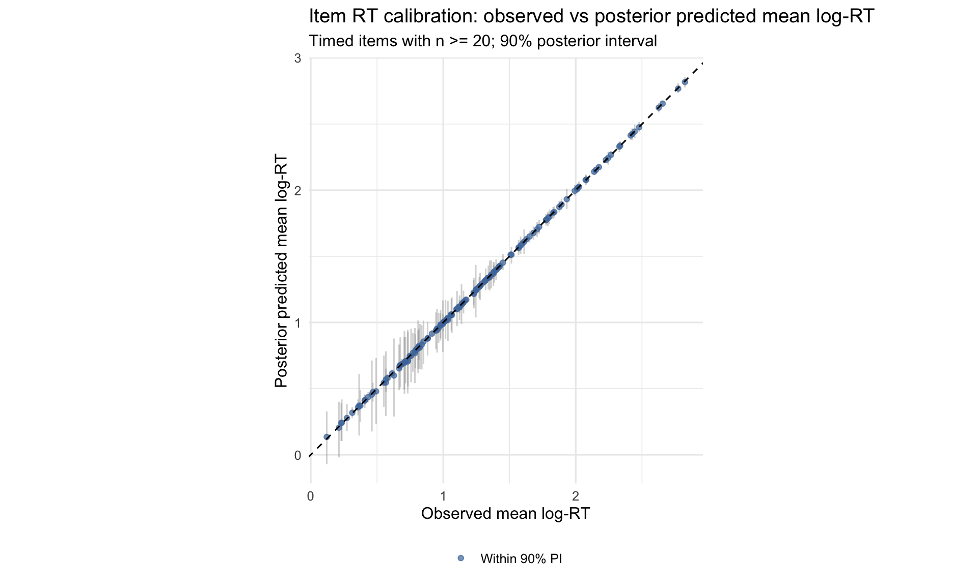
Interpretation: each point is an item’s observed mean log-RT (x) compared to the model-predicted mean log-RT (y), with a 90% predictive interval. Dots far from the diagonal or outside the interval flag items whose time intensity is not well captured (interpret only for items with n ≥ 20).
7.8.5 Joint speed–accuracy checks
These checks evaluate whether the joint model reproduces fast-wrong and fast-correct rates for timed-math subtests (Term 1 only), using posterior predictive simulations of both accuracy and RT.
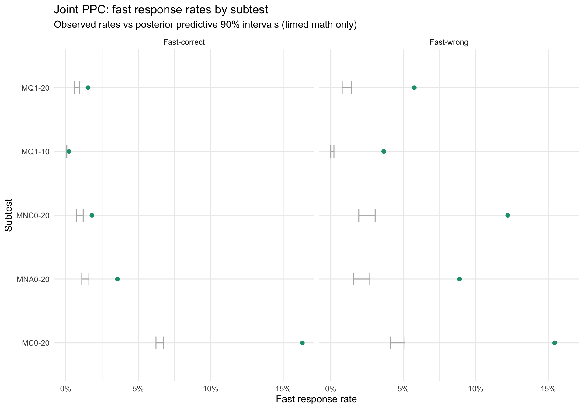
Interpretation: these panels compare observed fast-correct and fast-wrong rates (≤ 1s) to model-implied intervals. Large observed fast-wrong rates above the predictive interval suggest a rapid-guess / accidental-tap process that this v3 RT likelihood does not represent. This is a primary motivation for probe-aware RT modelling (e.g., correct-only RT for affected probes) in the next iteration.
8 Model Diagnostics
8.1 Input coverage (Foundation)
| year_level | n_rows | n_persons | n_acc_items | n_acc_bin | n_acc_nl | n_rt_items | n_rt_obs |
|---|---|---|---|---|---|---|---|
| foundation | 200822 | 2517 | 214 | 106479 | 46060 | 184 | 131978 |
8.2 Sampler diagnostics
| Metric | Value |
|---|---|
| Divergences | 0.000 |
| Treedepth hit rate | 0.000 |
| Max Rhat (key params) | 1.009 |
| Min ESS (key params) | 407.122 |
| Max Rhat (theta) | 1.004 |
| Min ESS (theta) | 5273.110 |
| Max Rhat (tau_base) | 1.004 |
| Min ESS (tau_base) | 5326.209 |
| Max Rhat (tau_math_total) | 1.004 |
| Min ESS (tau_math_total) | 5778.137 |
| Max Rhat (item params) | 1.007 |
| Min ESS (item params) | 557.667 |
| Min E-BFMI | 0.654 |
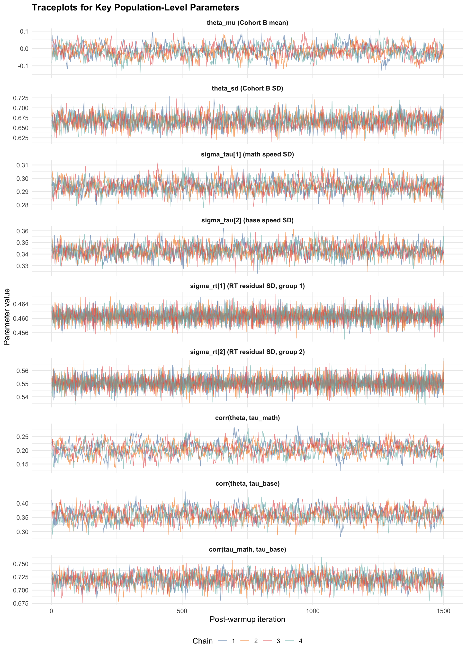
Diagnostics are clean (0 divergences; Rhat ≈ 1; strong ESS; healthy E-BFMI). Note that the JSON stores QC metadata from the QC run environment; the actual fit used 1500 warmup + 1500 sampling per chain.
8.3 Traceplots
Traceplots for key population-level parameters across all chains. Healthy mixing appears as overlapping, stationary traces with no trends or stuck regions.
8.4 Prior vs posterior overlap (key hyperparameters)
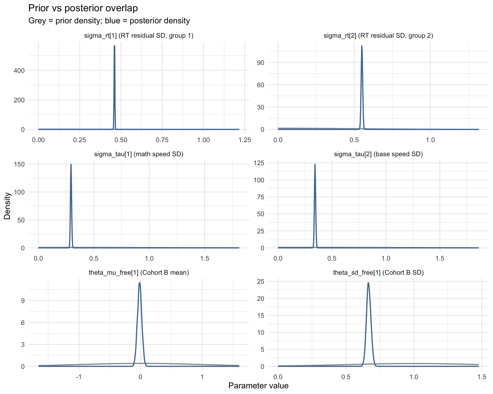
These overlays check whether the data meaningfully update the priors for core scale and linking parameters. Posteriors that closely match priors indicate weak identification.
8.5 RT preprocessing (floor/cap)
| test_subgroup | n_rt | n_included | n_floored | n_capped | p_floored | p_capped |
|---|---|---|---|---|---|---|
| MC0-20 | 40402 | 40402 | 4 | 1 | 1e-04 | 0.0000 |
| MNA0-20 | 7758 | 7758 | 1 | 1 | 1e-04 | 0.0001 |
| MNC0-20 | 7445 | 7445 | 0 | 2 | 0e+00 | 0.0003 |
| MQ1-10 | 17809 | 17809 | 0 | 9 | 0e+00 | 0.0005 |
| MQ1-20 | 10281 | 10281 | 0 | 50 | 0e+00 | 0.0049 |
| STPM | 48283 | 48283 | 0 | 285 | 0e+00 | 0.0059 |
Flooring is negligible and capping is rare, concentrated where expected (STPM has the largest share of long pauses).
8.6 Low-information flags
| year_level | low_info_n | low_info_rate | low_acc_items_rate | low_timed_math_rt_rate | low_speed_rt_rate | low_theta_precision_rate | low_tau_reg_precision_rate |
|---|---|---|---|---|---|---|---|
| foundation | 61 | 0.024 | 0.01 | 0.019 | 0.011 | 0.001 | 0 |
Low-information flags are rare (about 2.4%) and are driven by low item/RT counts rather than unstable posterior uncertainty.
8.7 Item-level QC notes
8.7.1 Low-exposure items
| n_items | n_low_n | pct_low_n | obs_low_n | obs_total | obs_share |
|---|---|---|---|---|---|
| 214 | 36 | 16.822 | 269 | 152539 | 0.002 |
| item_id | test_subgroup | n_total | b_mean | b_sd |
|---|---|---|---|---|
| MC0-20__MC0-20_044 | MC0-20 | 1 | -0.506 | 1.327 |
| MNC0-20__MNC0-20_030 | MNC0-20 | 1 | -0.782 | 1.285 |
| MNC0-20__MNC0-20_028 | MNC0-20 | 2 | 0.973 | 1.207 |
| MNC0-20__MNC0-20_026 | MNC0-20 | 2 | 1.091 | 1.202 |
| MNA0-20__MNA0-20_029new | MNA0-20 | 2 | -0.148 | 1.136 |
| MNC0-20__MNC0-20_029 | MNC0-20 | 2 | -1.651 | 1.133 |
| MNA0-20__MNA0-20_030new | MNA0-20 | 2 | -0.155 | 1.103 |
| MNC0-20__MNC0-20_027 | MNC0-20 | 3 | 1.190 | 1.138 |
| MNA0-20__MNA0-20_027new | MNA0-20 | 3 | 0.230 | 1.006 |
| MNC0-20__MNC0-20_025 | MNC0-20 | 3 | -0.989 | 0.995 |
| MNA0-20__MNA0-20_028new | MNA0-20 | 3 | -0.778 | 0.993 |
| MC0-20__MC0-20_042 | MC0-20 | 4 | -1.300 | 1.127 |
| MC0-20__MC0-20_041 | MC0-20 | 4 | -1.281 | 1.102 |
| MC0-20__MC0-20_039 | MC0-20 | 4 | -1.278 | 1.098 |
| MC0-20__MC0-20_043 | MC0-20 | 4 | -1.281 | 1.090 |
These low-n items represent a tiny share of all accuracy observations, so they have limited impact on student scores but should be filtered in any item-level ranking or review.
8.7.2 Number-line step ordering
| n_items | n_ordered | pct_ordered |
|---|---|---|
| 30 | 27 | 90 |
| item_id | test_subgroup | step1_step_mean | step2_step_mean |
|---|---|---|---|
| BNL0-20__BNL0-20_008new-copy | BNL0-20 | 0.156 | -0.156 |
| UNLC0-20__UNLnc0-20_005-copy | UNLC0-20 | 0.209 | -0.209 |
| UNLNC0-20__UNLnc0-20_005-copy | UNLNC0-20 | 0.671 | -0.671 |
For 3-category PCM, ordered steps are expected. A small subset of NL items show disordered steps; these are targeted candidates for review rather than a threat to overall model stability.
8.8 Pending item review
The following item-level review tasks remain outstanding:
- Outfit / infit statistics: Compute and review item fit indices to identify items performing worse than expected under the Rasch/PCM model.
- Differential item functioning (DIF): Test whether items function equivalently across cohorts A and B.
- Anchor item residuals: Assess stability of shared items used for cohort linking.
The flags identified in this report — low-exposure items (n < 20) and NL step disorder — are review flags, not automatic retirement triggers. They identify items to inspect for scoring, coding, or form assignment issues before any change to the instrument.
9 Lessons Learnt & Implications for Next Iteration
This section collects findings from the Foundation Term 1 review that inform future modelling decisions. It is intended as a working reference for the next calibration cycle.
9.1 What worked well
- Accuracy model convergence: 0 divergences, healthy ESS across all parameters, max Rhat ~1.01, E-BFMI well above warning thresholds. The Rasch (1PL) + PCM specification is well-identified for this dataset.
- Construct validity: θ aligns strongly with observed accuracy; τ_base tracks STPM speed; τ_math_total tracks timed-math speed; τ_reg_adj is approximately independent of baseline speed. The latent traits behave as intended.
- Binary item calibration: 0/184 items outside the 90% posterior predictive interval for observed proportion correct. In-sample calibration is tight.
- Prior calibration: posteriors are narrower than priors for all key hyperparameters, indicating that the data are informative and the priors are not unduly constraining estimates.
9.2 What needs attention
- Fast-wrong responses not modelled: v3 includes all attempted RTs. Observed fast-wrong rates exceed PPC intervals for timed-math subtests (MC0-20, MNC0-20). Speed scores for students with many fast-wrong responses may be biased upward (faster apparent speed from rapid guesses rather than fluent retrieval).
- STPM 60-second cap rate: the observed cap rate far exceeds the model’s 90% PI. Capped RTs are treated as exact observations (log(60)), which biases τ_base downward (slower apparent speed) for affected students.
- Heavy RT tails: p99 quantiles are systematically underpredicted — the lognormal residual is too thin-tailed at the extremes, even where the bulk of the distribution fits well.
- PPC plumbing matters: PPCs are only as reliable as their indexing/aggregation. Keep Stan matrix reshaping consistent with Stan’s column-major order, and ensure group aggregation preserves ordering (avoid
rowsum(..., reorder = FALSE)when results are later aligned to numeric IDs). - PPC total score definition: the current PPC sums binary 0/1 accuracy scores with NL category scores (0/1/2). This is a valid internal consistency check but does not correspond to an operational reporting metric. Future PPCs should consider separate accuracy-only and NL-only checks to avoid conflating different scoring scales.
9.3 Recommendations for next iteration
9.3.1 Immediate (v4 changes)
- Correct-only RT filtering for flagged subtests. Apply a probe-aware RT inclusion policy for timed-math subtests with high fast-wrong rates/excess (e.g., MC0-20, MNC0-20). This targets the primary source of RT misfit without discarding accuracy data.
- Document the RT filtering policy as a formalised pre-model data step with auditable thresholds (e.g., percentage of fast-wrong responses triggering correct-only mode for a subtest), and lock the resulting policy table per run_id.
- Add speed reliability flags for reporting/operations (e.g., min number of correct RTs, STPM cap hits, fast-wrong excess) so speed scores can be downweighted or withheld when not informative.
9.3.2 Medium-term (model extensions)
- Censored or mixture model for 60-second cap. Right-censoring is the cleanest fix for cap-rate misfit — it tells the model “this student’s true RT is ≥60s” rather than “this student’s true RT is exactly 60s.” A mixture model is more complex but could target both p99 and cap-rate misfit simultaneously.
- Heavier-tailed RT residual (Student-t with df = 5–10) if p99 underprediction persists after correct-only filtering. The lognormal assumption is adequate for the bulk of the distribution but fails at the extremes.
9.3.3 Deferred
- Item-fit, DIF, and local dependence checks remain outstanding (see Pending Item Review above). These are necessary before any high-stakes use of item parameters.
- Cross-validate PPC total score definition — investigate whether any observed mean/SD shift persists after PPC plumbing audits. The total score density overlay is the more robust check; mean/SD deviations may be a definitional artefact of mixing binary and ordinal scoring scales rather than genuine model misfit.
10 (APPENDIX) Appendix: Reproducibility
10.1 Run Metadata
| Field | Value |
|---|---|
| Run ID | t1_2025_joint_flu_v1 |
| Model root | models/irt/irt_joint_stan_pcm |
| R Version | 4.5.2 |
| cmdstanr Version | 0.9.0 |
| Report Generated | 2026-02-03 01:49:23.856953 |
10.2 File Paths
| File | Path |
|---|---|
| Cleaned responses | data/processed/cleaned_responses/cleaned_responses.parquet |
| Student scores | models/irt/irt_joint_stan_pcm/outputs/runs/t1_2025_joint_flu_v1/final/students/term1_joint_scores_foundation.csv |
| Item parameters | models/irt/irt_joint_stan_pcm/outputs/runs/t1_2025_joint_flu_v1/final/items/term1_joint_item_params_foundation.csv |
| Model diagnostics (sampler) | models/irt/irt_joint_stan_pcm/outputs/runs/t1_2025_joint_flu_v1/qc/sampler_diagnostics_foundation.json |
| Model summary | models/irt/irt_joint_stan_pcm/outputs/runs/t1_2025_joint_flu_v1/qc/term1_joint_summary_foundation.csv |
| Low-information summary | models/irt/irt_joint_stan_pcm/outputs/runs/t1_2025_joint_flu_v1/qc/term1_joint_low_info_foundation.csv |
| RT preprocessing summary | models/irt/irt_joint_stan_pcm/outputs/runs/t1_2025_joint_flu_v1/qc/term1_rt_preproc_foundation.csv |
| Stan data (foundation) | models/irt/irt_joint_stan_pcm/outputs/runs/t1_2025_joint_flu_v1/intermediate/term1_joint_stan_data_foundation.rds |
10.3 Known Quirks & Limitations
- UNLC/UNLNC variants: Form-confounded (chair vs no-chair), NOT true anchors
- Reach analysis: Deferred; gap/tail classification is a proxy only
- RT censoring: Not modelled; 60s cap may truncate valid slow responses
- NL step disorder: A small subset of NL items show disordered PCM steps; these items should be reviewed for scoring/calibration issues
- Low-n items: Parameter estimates for items with <20 responses are unstable and should be filtered from item-level rankings
- Untimed RT: Excluded from baseline model; 180s cap used in sensitivity runs only