Outcome Pack Comparison: Preparing Benchmark Data for Screener Prediction
Pack A (Strict) vs Pack B (Full Coverage)
1 Purpose and Overview
An outcome pack is a scored dataset containing latent attainment estimates (η) and risk probabilities for each student, derived from PAT scores and teacher achievement ratings. It serves as the benchmark target for screener-based prediction models.
Two outcome packs are compared here:
| Pack | Scope | Description |
|---|---|---|
| A | Strict | Model fit restricted to students in schools with type-gated PAT. Includes PAT-backed students plus rating-only students in those same schools. |
| B | Full coverage | Model fit uses all students with any outcome evidence: type-gated PAT plus all teacher ratings regardless of school PAT availability. |
Both packs use the same Bayesian joint measurement model and scoring pipeline; they differ only in which students enter the model fit.
1.1 PAT Score vs Provided Percentile
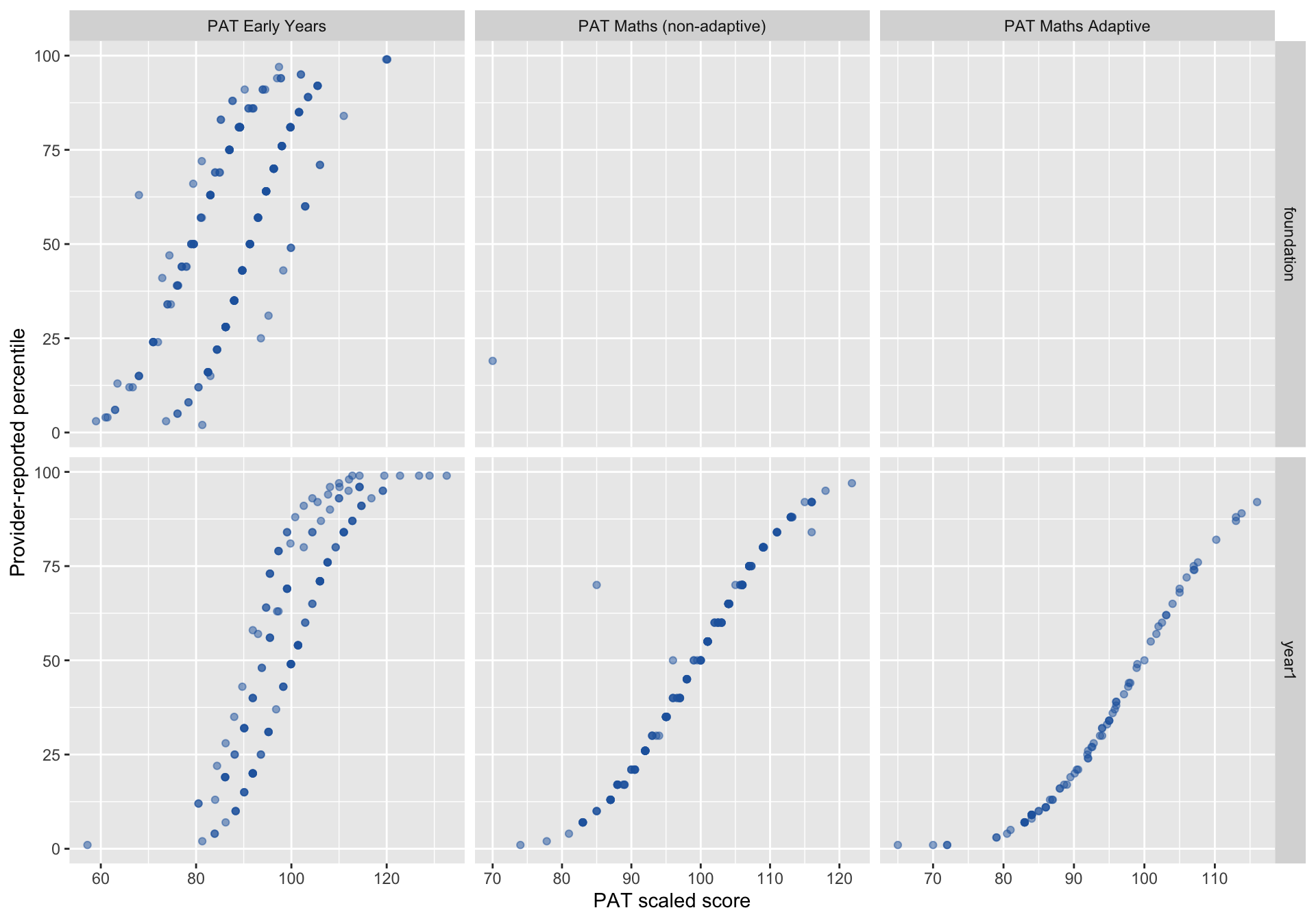
Before comparing packs, we examine a data quality issue that motivates the anchor-truth policy used in Section 6. Each dot is one PAT record. If percentiles were correctly assigned, dots would form a smooth upward curve. Where they scatter or reverse direction, the percentile mapping is unreliable — meaning we cannot simply use “percentile ≤ 25” to define who is truly below the 25th percentile.
Note
For PAT Early Years in Foundation (Oct–Dec administration window), the relationship between scaled score and provider-reported percentile shows non-monotonic regions, indicating internal inconsistency in the percentile mapping. This motivates the hybrid anchor-truth policy described in Section 6.
2 Model Specification — Pack A vs Pack B
2.1 Type Gate
The type gate restricts which PAT types enter the model. PAT Maths Adaptive is excluded because of norm-frame incompatibility with the joint model’s measurement equation.
| Field | Value |
|---|---|
| Included PAT types | PAT Early Years, PAT Maths (non-adaptive), PAT type missing |
| Excluded PAT types | PAT Maths Adaptive |
2.2 Joint Measurement Model
Both packs use the same Bayesian model — a single latent construct η (end-of-year maths attainment, in PAT scale-score units) measured through two instruments:
PAT measurement equation (students with PAT scores):
\[\text{PAT}_{ij} \sim \text{Normal}\!\left(\eta_i + \delta_{\text{type}[j]},\; \sqrt{\sigma^2_{\text{pat}} + \sigma^2_{\text{time}} \cdot \Delta t_{ij}^2 + \text{SE}^2_{\text{cond}[ij]}}\right)\]
Teacher rating equation (students with achievement ratings):
\[\text{Rating}_i \sim \text{OrderedLogistic}(\alpha + \lambda \, \eta_i, \; \tau)\]
Prior on student attainment:
\[\eta_i \sim \text{Normal}(\mu_{\text{yr}},\; \sigma_\eta)\]
In plain terms:
- η is what we are estimating — each student’s underlying maths attainment at end-of-year, expressed in PAT scale-score units (~50–150).
- δtype captures systematic offsets between PAT products (e.g. PAT Early Years vs PAT Maths non-adaptive). Different tests can give slightly different readings of the same ability.
- σtime · Δt inflates uncertainty for PAT scores administered further from end-of-year. A test taken in August is less informative about December attainment than one taken in November.
- SEcond is the conditional standard error reported by ACER for each PAT record — known measurement noise baked into the likelihood.
- λ (lambda) links the teacher rating scale to the PAT scale. It translates from “scale-score units” to “how much the rating moves per unit of attainment.”
- τ (tau) are ordered thresholds defining the boundaries between rating categories 1–5.
TipWhat differs between Pack A and Pack B?
The model specification is identical. The only difference is which students are included in the fit:
- Pack A restricts to students in schools that have type-gated PAT, so the model sees both PAT and rating evidence from the same school context.
- Pack B includes all students with any outcome evidence, adding rating-only students from non-PAT schools.
Pack B’s broader sample may improve precision for the rating pathway but could introduce school-level confounding if rating cultures differ systematically between PAT-backed and non-PAT schools.
2.3 Eligibility Breakdown (Pack A)
| Eligibility reason | n | % |
|---|---|---|
| No_outcome_data | 5561 | 69.8% |
| Rating_only_non_pat_school | 1813 | 22.7% |
| Both | 431 | 5.4% |
| Rating_only_in_pat_backed_school | 114 | 1.4% |
| PAT_only | 52 | 0.7% |
2.4 Composition Summary
| Pack | n | Foundation | Year 1 | Inconclusive | % inconclusive |
|---|---|---|---|---|---|
| A | 597 | 281 | 316 | 138 | 23.1% |
| B | 2410 | 1166 | 1244 | 232 | 9.6% |
TipWhat does “inconclusive” mean?
Inconclusive is a governance policy, not a model output. A student is flagged inconclusive when:
- Their posterior standard error exceeds the 95th percentile threshold, or
- Their PAT timing distance exceeds 150 days from the end-of-year reference.
These students receive η estimates but are excluded from operational risk classification.
2.5 Source Composition
| Source | Pack A | Pack B |
|---|---|---|
| Both | 431 | 431 |
| PAT only | 52 | 52 |
| Rating only | 114 | 1927 |
3 Distributions
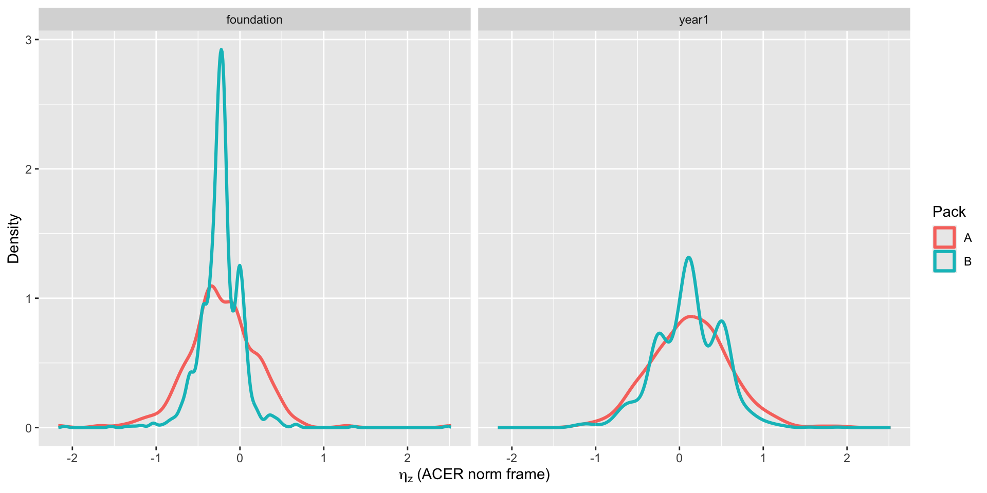
3.1 Latent Attainment (ηz)
This shows the spread of estimated attainment within each year level. ηz is a z-score: 0 means the ACER national average, negative values are below average. Faceting by Foundation and Year 1 avoids pooled-shape artefacts and makes Pack A vs Pack B comparisons interpretable within cohort.
3.2 Tail Probability: P(η < P25)
For each student, the model produces a probability of being below the 25th percentile. Most students cluster near 0% (unlikely to be at risk) or near 100% (very likely at risk). Students in between are the “borderline zone” where classification is least certain.

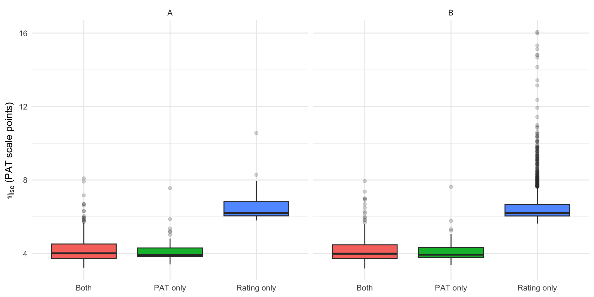
3.3 Uncertainty by Source
Rating-only students (no PAT score) have higher uncertainty than students with PAT data. Students with both sources (“Both”) tend to have the lowest uncertainty. This plot shows why having PAT data matters for precision — and why Pack B’s additional rating-only students come with a cost in confidence.
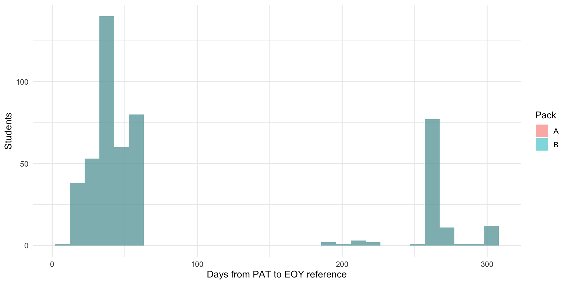
3.4 PAT Timing Distance
PAT tests taken further from the end-of-year reference date carry more uncertainty because students may have grown in the interim. This histogram shows how many days separated each PAT administration from the reference date. A tight cluster near zero is ideal.
4 Coherence Checks
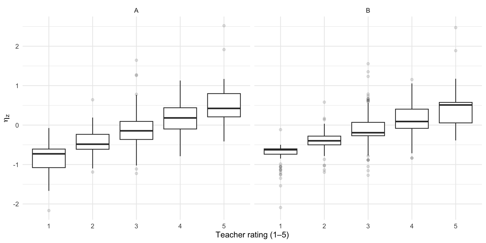
4.1 Teacher Rating vs ηz
If the model is sensible, students rated higher by their teacher should also have higher estimated attainment. The boxplots should step upward from rating 1 to rating 5. Overlap between adjacent boxes is expected — ratings are coarse.
4.2 Spearman Correlations
Spearman rank correlations quantify the monotonic agreement between teacher ratings and model estimates. Values near −1 or +1 indicate strong agreement; near 0 indicates no relationship. A negative correlation with P(η < P25) is expected — higher-rated students should have lower risk probability.
| Pack | n | ρ (rating, η_z) | ρ (rating, P25) |
|---|---|---|---|
| A | 545 | 0.535 | -0.452 |
| B | 2358 | 0.673 | -0.616 |
4.3 ACER Risk Band Distribution
Students are classified into High, Moderate, or Low risk using ACER national norms. This table shows how many students fall into each band under each pack.
| ACER risk band | Pack A | Pack B |
|---|---|---|
| High | 3 | 3 |
| Moderate | 17 | 26 |
| Low | 577 | 2381 |
5 Pack A vs Pack B Sensitivity (Overlap Students)
Pack A and Pack B are separate model fits. To assess sensitivity to the sample composition, we compare estimates for the overlapping student set (students in both packs). High correlations and low MAE indicate that the choice between Pack A and Pack B has little practical effect on individual student estimates. Systematic differences would appear as points deviating from the dashed diagonal.
5.1 Correlation and Agreement
| Metric | Value |
|---|---|
| n overlap | 597 |
| Pearson (η̂) | 0.9986 |
| Spearman (η̂) | 0.9984 |
| MAE (η̂) | 0.277 |
| Pearson (P25) | 0.9962 |
| Spearman (P25) | 0.9971 |
| MAE (P25) | 0.0098 |
5.2 η̂ Scatter (A vs B)
Each dot is one student. Points close to the dashed line received similar η̂ estimates under both packs. Systematic departures from the diagonal would suggest the additional students in Pack B are pulling estimates in a particular direction.

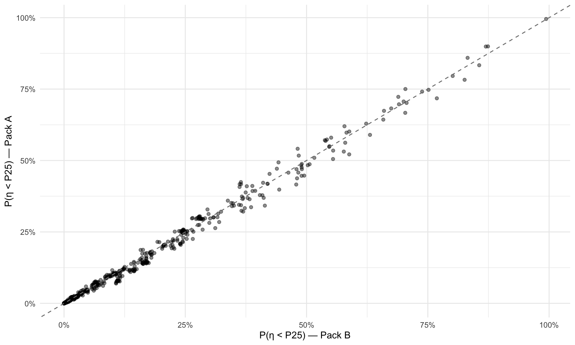
5.3 P(η < P25) Scatter (A vs B)
Same as above but for the risk probability. Points in the upper-left or lower-right corners would indicate students whose risk classification flips between packs.
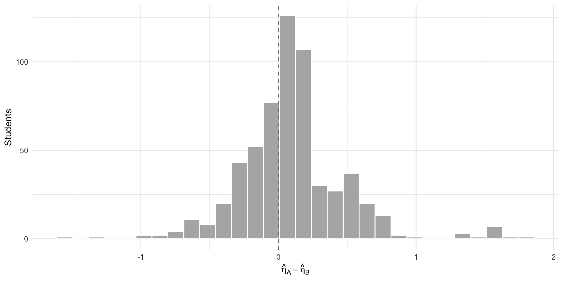
5.4 η̂ Difference Distribution
The distribution of Pack A minus Pack B η̂ values. A distribution centred on zero with small spread means the two packs produce practically interchangeable estimates.
6 PAT-Anchor Benchmark
This section evaluates how well the outcome pack’s risk probabilities align with an external anchor: PAT-derived “below P25” status. This is the primary validation available before screener-level external validation data arrives.
6.1 Why PAT Percentile as “Truth” Is Non-Trivial
PAT Early Years percentiles show internal incoherence — the provided percentile does not always increase monotonically with the scaled score (see Section 1.1). This means we cannot naively use the provider-reported percentile to define “truly below P25” for all students.
The hybrid anchor-truth policy resolves this:
| PAT type × year level | Anchor truth method | Rationale |
|---|---|---|
| PAT Maths (non-adaptive), Year 1 | Percentile ≤ 25 | Monotonic score-percentile relationship |
| PAT Maths (non-adaptive), Foundation | Scale-cut fallback | Sparse data, percentile unreliable |
| PAT Early Years, Foundation | Scale-cut fallback | Non-monotonic percentile mapping |
| PAT Early Years, Year 1 | Scale-cut fallback | Cross-year norm frame issues |
Row-level safeguard: Even where percentile is used as anchor truth, PAT Maths records with empirical residual > 15 fall back to scale-cut to guard against individual anomalous mappings.
6.2 Anchor Truth Provenance
The table below shows how many students had their “truth” status determined by each method. Because PAT Early Years dominates this cohort and its percentiles are unreliable, most students fall back to the scale-cut method.
| Anchor truth source | n | % |
|---|---|---|
| percentile | 142 | 38.2% |
| scale_cut_fallback_frame | 229 | 61.6% |
| scale_cut_fallback_impossible_pair | 1 | 0.3% |
| Anchor truth source | n | % |
|---|---|---|
| percentile | 28 | 16.4% |
| scale_cut_fallback_frame | 143 | 83.6% |
Note
Most anchor truth comes from the scale-cut fallback because PAT Early Years — the dominant PAT type in this cohort — has unreliable percentile mappings. The scale-cut method uses year-level-specific η cutpoints instead of provider percentiles.
6.3 Confusion Matrix vs PAT Anchor Truth
The table below shows classification performance at each candidate operating threshold, stratified by year level. The model’s P(η < P25) is thresholded and compared against PAT-anchored truth. Read this table as: at threshold 0.6, if the model says a student has ≥60% probability of being below P25, how often is PAT anchor truth confirming that? Precision = of those flagged, how many truly are below P25. Recall = of those truly below P25, how many did the model catch.
| Threshold | Year level | n | TP | FP | FN | TN | Precision | Recall | Specificity |
|---|---|---|---|---|---|---|---|---|---|
| 0.5 | foundation | 108 | 13 | 3 | 11 | 81 | 0.812 | 0.542 | 0.964 |
| 0.5 | year1 | 63 | 8 | 0 | 7 | 48 | 1.000 | 0.533 | 1.000 |
| 0.6 | foundation | 108 | 9 | 0 | 15 | 84 | 1.000 | 0.375 | 1.000 |
| 0.6 | year1 | 63 | 8 | 0 | 7 | 48 | 1.000 | 0.533 | 1.000 |
| 0.7 | foundation | 108 | 5 | 0 | 19 | 84 | 1.000 | 0.208 | 1.000 |
| 0.7 | year1 | 63 | 8 | 0 | 7 | 48 | 1.000 | 0.533 | 1.000 |
| 0.8 | foundation | 108 | 3 | 0 | 21 | 84 | 1.000 | 0.125 | 1.000 |
| 0.8 | year1 | 63 | 3 | 0 | 12 | 48 | 1.000 | 0.200 | 1.000 |
| Threshold | n operational | n high-flag | % high-flag | n review | % review | n PAT-anchored | Precision (PAT) | Recall (PAT) |
|---|---|---|---|---|---|---|---|---|
| 0.5 | 1657 | 288 | 17.4% | 0 | 0.0% | 171 | 0.875 | 0.538 |
| 0.6 | 1657 | 85 | 5.1% | 203 | 12.3% | 171 | 1.000 | 0.436 |
| 0.7 | 1657 | 68 | 4.1% | 220 | 13.3% | 171 | 1.000 | 0.333 |
| 0.8 | 1657 | 12 | 0.7% | 276 | 16.7% | 171 | 1.000 | 0.154 |
Tip
The selected operating threshold of 0.6 achieves precision = 1.00 (no false positives among PAT-anchored students) with recall = 0.44 (catches 44% of PAT-confirmed below-P25 students). The conservative precision reflects the governance priority: avoid mislabelling students as at-risk when external evidence does not support it.
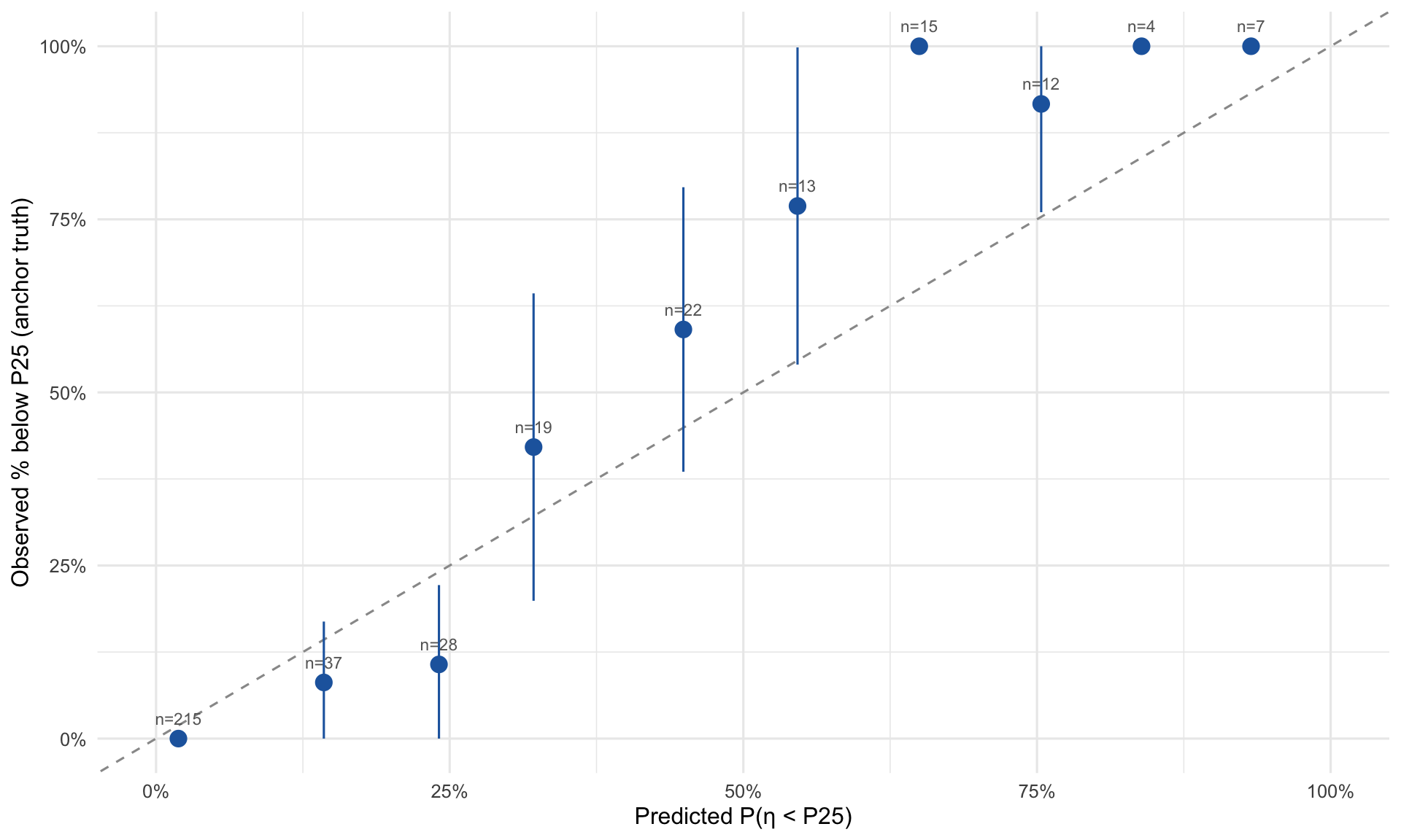
6.4 Calibration View
Does the model’s stated probability track observed reality? Below, students are binned by their predicted P(η < P25) and we plot the observed proportion with anchor truth confirming below-P25 status. If the model is well-calibrated, points should lie on the dashed diagonal — e.g., among students the model gives a 40% risk probability, roughly 40% should actually be below P25 according to anchor truth. Points above the diagonal mean the model underestimates risk; below means it overestimates.
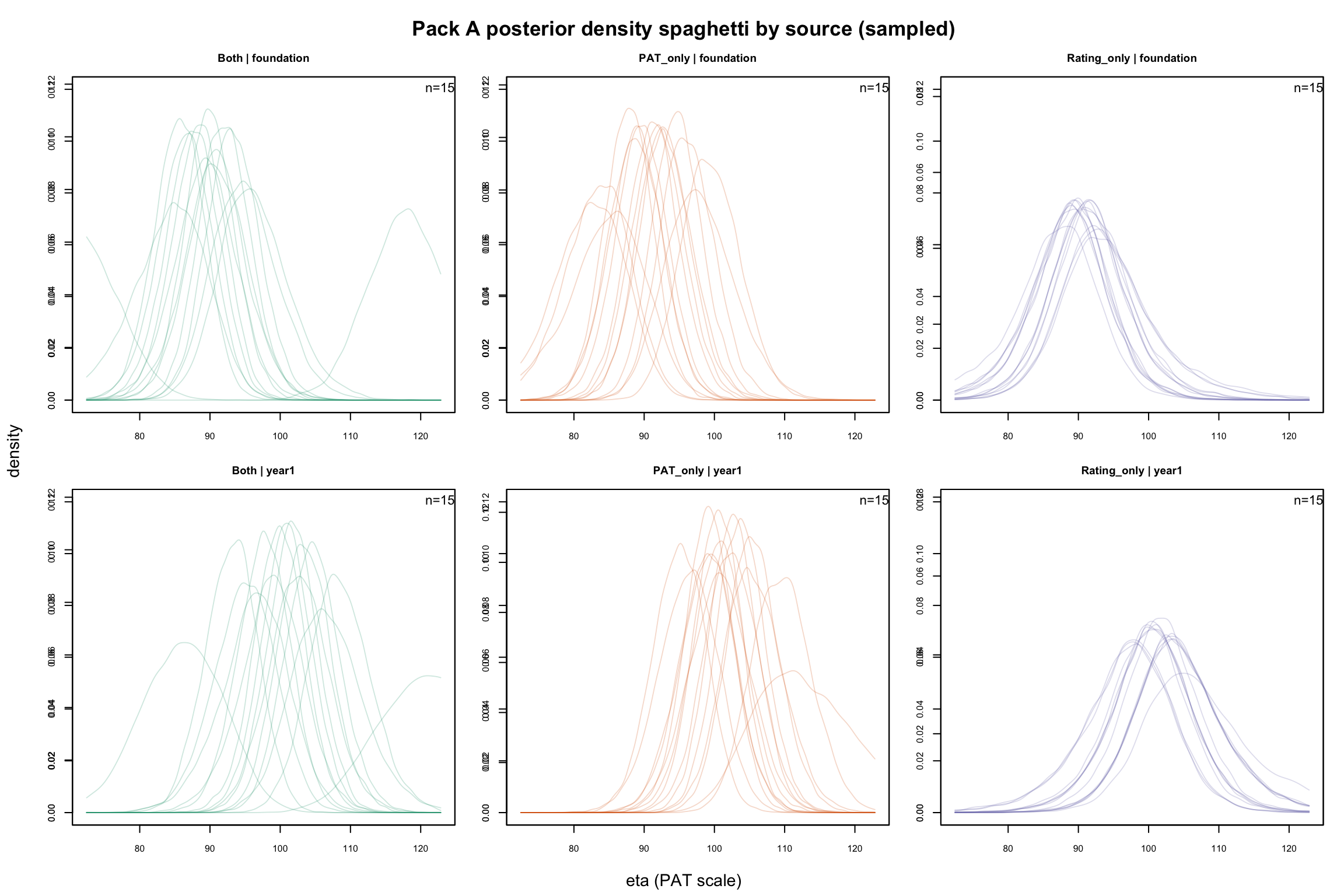
7 Appendix: Pack A Posterior Diagnostics
These plots visualise sampled posterior densities for student-level η from the Pack A Bayesian fit. They serve as qualitative diagnostics for posterior shape, separation, and uncertainty — not as a primary reporting view.
7.1 By Source Flag
Each translucent curve is one student’s posterior density — the model’s belief about where that student’s true attainment lies. Wider curves mean more uncertainty. Compare across panels: rating-only posteriors (purple) are typically wider than PAT-backed posteriors (orange/green).
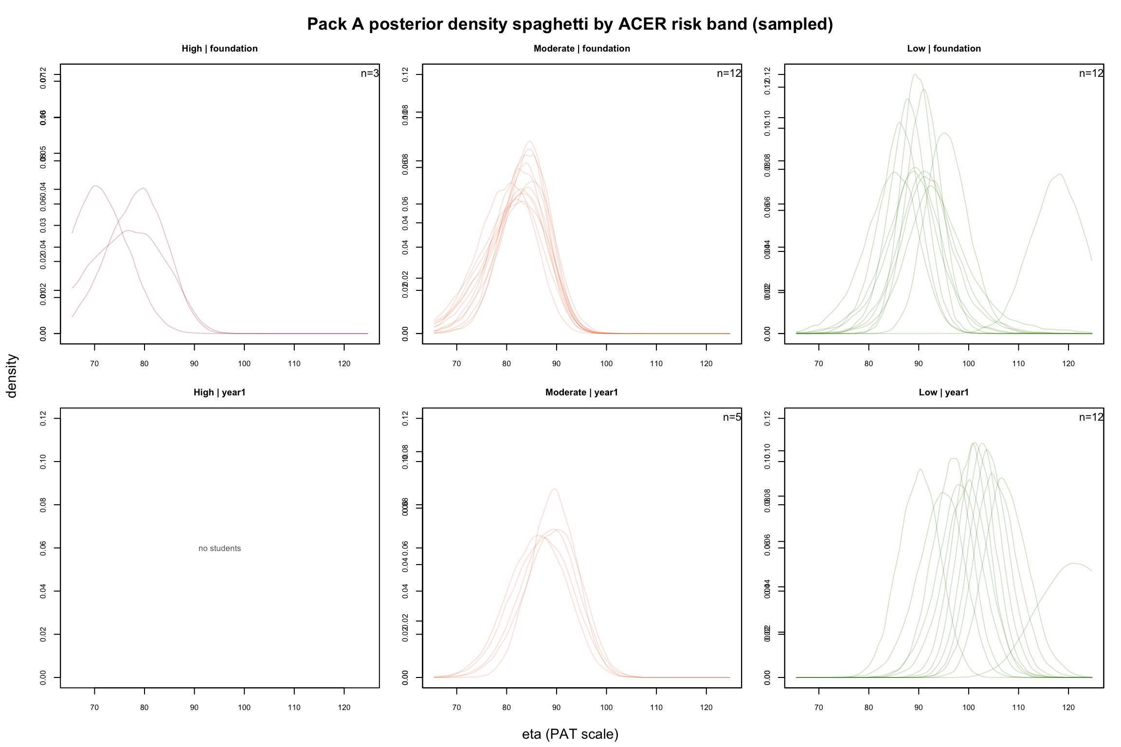
7.2 By ACER Risk Band
Same idea, but students are grouped by ACER risk band. High-risk posteriors (red) should cluster at lower η values; Low-risk posteriors (green) should cluster higher. Overlap between bands in the same year level indicates the borderline zone.